1 Introduction to APP4MC

The goal of the project is the development of a consistent, open, expandable tool platform for embedded software engineering. It is based on the model driven approach as basic engineering methodology. The main focus is the optimization of embedded multi-core systems.
Most functions in a modern car are controlled by embedded systems. Also more and more driver assistance functions are introduced. This implies a continuous increase of computing power accompanied by the request for reduction of energy and costs. To handle these requirements the multi-core technology permeates the control units in cars. This is today one of the biggest challenges for automotive systems. Existing applications can not realize immediate benefit from these multi-core ECUs because they are not designed to run on such architectures. In addition applications and systems have to be migrated into AUTOSAR compatible architectures. Both trends imply the necessity for new development environments which cater for these requirements.
The tool platform shall be capable to support all aspects of the development cycle. This addresses predominantly the automotive domain but is also applicable to telecommunication by extensions which deal with such systems in their native environment and integrated in a car.
Future extensions will add support for visualization tools, graphical editors. But not only design aspects will be supported but also verification and validation of the systems will be taken into account and support tools for optimal multi-core real-time scheduling and validation of timing requirements will be provided. In the course of this project not all of the above aspects will be addressed in the same depth. Some will be defined and some will be implemented on a prototype basis. But the basis platform and the overall architecture will be finalized as much as possible.
The result of the project is an open tool platform in different aspects. On the one hand it is published under the Eclipse Public License (EPL) and on the other hand it is open to be integrated with existing or new tools either on a company individual basis or with commercially available tools.
2 User Guide
2.1 Introduction
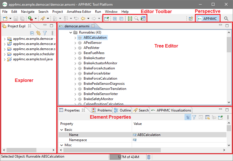
APP4MC comes with a predefined perspective available in the Eclipse menu under Window -> Open Perspective -> Other -> APP4MC. This perspective consists of the following elements:
- Project Explorer
- Editor
- Tree Editor showing the structure of the model content
- Standard Properties Tab is used to work on elements attributes
The following screenshot is showing this perspective and its contained elements.
2.1.1 Steps to create a new AMALTHEA model
APP4MC provides a standard wizard to create a new AMALTHEA model from scratch.
Step 1: Create a new general project
The scope of an AMALTHEA model is defined by its enclosing container (project or folder).
Therefore a project is required.
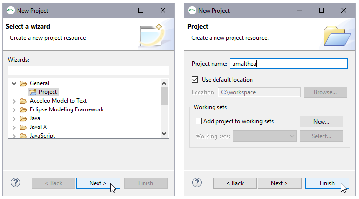
Step 2: Create a new folder inside of the created project
It is recommended to create a folder (
although a project is also a possible container ).
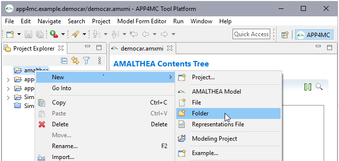
Step 3: Create a new AMALTHEA model
In the context menu (right mouse button) an entry for a new AMALTHEA model can be found.
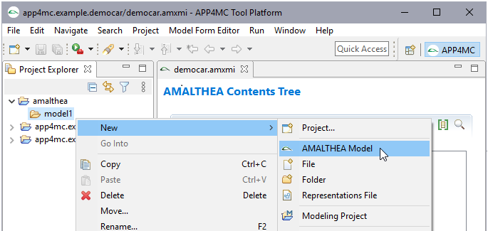
Another starting point is
File ->
New ->
Other
In the dialog you can select the parent folder and the file name.
2.1.2 AMALTHEA Editor
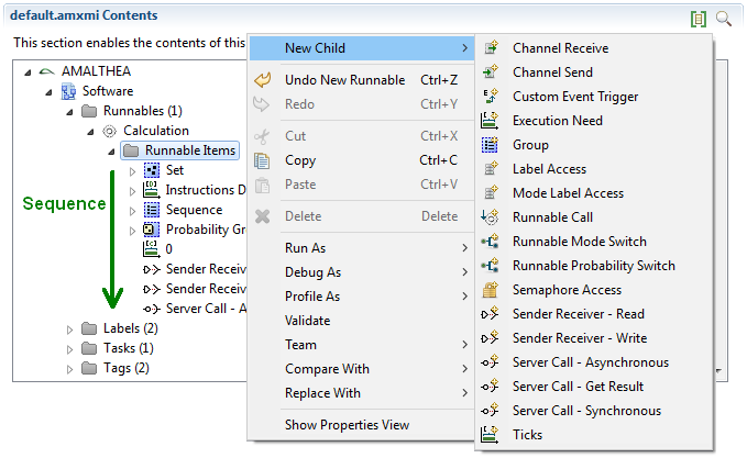
The AMALTHEA Editor shows the entire model that contains sub models.
The next screenshot shows the "New Child" menu with all its possibilities.
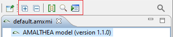
The AMALTHEA Editor has additional commands available in the editor toolbar.
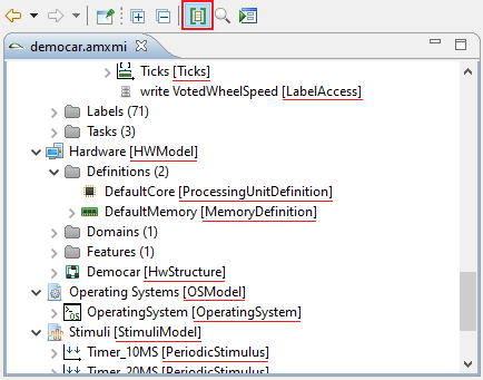
Show types of model elements
The Show types of elements button triggers the editor to show the direct type of the element in the tree editor using [element_type]. The following screenshot shows the toggle and the types marked with an underline.
Search for model elements
The editor provides the possibility to search for model elements by using the available name attribute. For example this can be used to find all elements in the model with "ABS" at the beginning of their name. The result are shown in the Eclipse search result view.
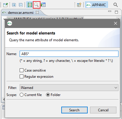
A double click on a result selects the element in the editor view.
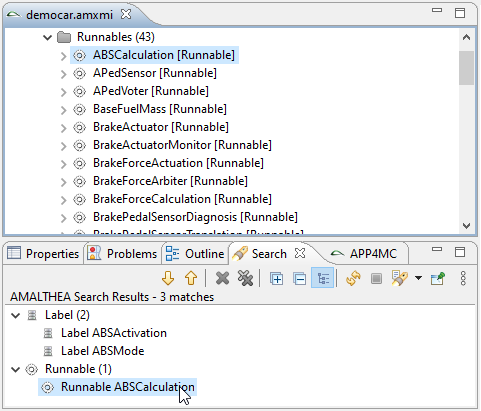
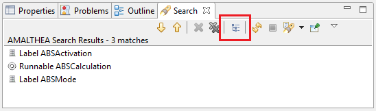
An additional option is to toggle the search results to show them as a plain list instead of a tree grouped by type.
2.1.3 Handling of multiple files (folder scope)
Amalthea model
- Amalthea files have the extension ".amxmi".
- Amalthea models support references to other model files in the same folder.
When the
first Amalthea file in a folder is opened in the Amalthea editor
- all valid model files are loaded
- a common editing environment is established
- files and folder are decorated with markers
- loaded model files are decorated with a green dot
- model files that contain older versions are extended with the version
- the folder is marked as "is in use" and decorated with a construction barrier
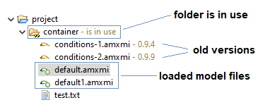
When the
last Amalthea editor of a folder is closed
- the common editing environment is released
- markers are removed
Warning:
Do not modify the contents of a folder while editors are open.
If you want to add or remove model files then first close all editors.
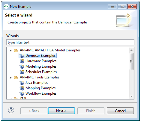
2.1.4 AMALTHEA Examples
The AMALTHEA tool platform comes with several examples. This section will describe how a new project based on these examples can be created.
Step 1
Click the "new" icon in the top left corner and select "Example..." or use the right mouse button.
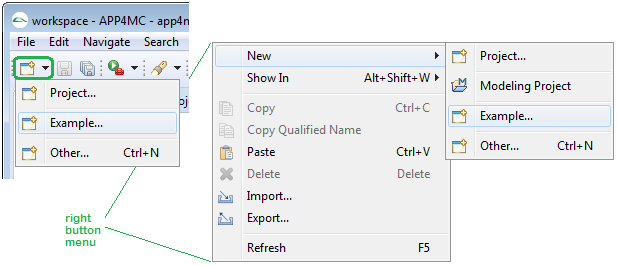
Step 2
The "New Example" wizard will pop up and shows several examples.
Select one examples and hit continue.
Step 3
You will see a summary of the example projects that will be created.
Click "Finish" to exit this dialog.
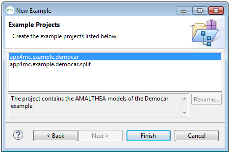
You can now open the editor to inspect the models.
2.2 Concepts
2.2.1 Timing in Amalthea Primer
An Amalthea model per se is a static, structural model of a hardware/software system. The basic structural model consists of software model elements (tasks, runnables), hardware model elements (processing units, memories, connection handlers), stimuli that are used to activate execution, and mappings of software model elements to hardware model elements. Semantics of the model then allows for definite and clear interpretation of the static, structural model regarding its behavior over time.
Different Levels of Model Detail
Amalthea provides a meta-model suitable for many different purposes in the design of hardware/software systems. Consequently, there is not
the level of Amalthea model detail – modeling often is purpose driven. Regarding timing analysis, we exemplary discuss three different levels of detail to clarify this aspect of Amalthea. Note that we focus on level of detail of the hardware model and assume other parts of the model (software, mapping, etc.) fixed.
Essential software model elements are runnables, tasks, and data elements (labels and channels). Runnable items of a runnable specifies its runtime behavior. You may specify the runnable items as a directed, acyclic graph (DAG). Amalthea has different categories of runnable items, we focus on the following four:
- Items that
branch paths of the DAG (runnable mode switch, runnable probability switch).
- Items that
signal or call other parts of the model (custom event trigger, runnable call, etc.).
- Items that specify
data access of data elements (channel receive/send, label access).
- Items that specify
execution time (ticks, execution needs).
Tasks may call runnables in a activity graph. Note that a runnable can be called by several tasks. We then map tasks to task schedulers in the operating system model, and we map every task scheduler to one or more processing units of the hardware model. Further, we map data elements to memories of the hardware model.
This coarse level of hardware model detail – the hardware model consists only of
mapping targets, without routing or timing for data accesses – may already be sufficient for analysis focusing on event-chains or scheduling.
As the second example of model detail, we now add access elements to all processing units of the hardware model,
modeling data access latencies or data rates when accessing data in memories – still ignoring routing and contention. This level of detail is sufficient, for example, for optimizing data placement in microcontrollers using static timing analysis.
A more detailed hardware model, our third and last example of model detail, will contain information about
data routing and congestion handling. Therefore, we add connection handlers to the hardware model for every possible contention point, we add ports to the hardware elements, and we add connections between ports. For every access element of the processing units, we add an access path, modeling the access route over different connections and connectionHandlers. The combination of all access elements are able to represent the full address space of a processing unit. This level of detail is well suited for dynamic timing simulation considering arbitration effects for data accesses.
In the following, we discuss 'timing' of Amalthea in context of level of detail of the last example and discrete-event simulation.
Discrete-Event Simulation
For dynamic timing analysis, the
initial state of the static system model is the starting point, and a series of
state changes is subject to model analysis. The
state of a model mainly consist of states of HW elements (processing units and connection handlers). During analysis, a state change is then, for example, a processing unit changing from
idle to
execute.
When we are interested in the
timing of a model, a common way is using discrete-event simulation. In discrete-event simulation, a series of
events changes the state of the system and a simulated clock. Such a simulation event is, for instance, a
stimuli event for a task to execute on a processing unit, what in turn may change the
state of this processing unit from
idle to
execute.
Note that every event occurs at a specified point in simulated time; for instance, think of a new
stimuli event that shall activate a task in 10ms from the current value of the simulated clock. Unprocessed (future) events are stored in an event list. The simulator then continuously processes the event occurring next to the current simulated time, and forwards the simulated clock correspondingly, thereby removing the event from the event list. Note that this is a very simplified description. For instance, multiple events at the same point in simulated time are possible. Processing events may lead to generation of new events. For instance, processing an end
task execution event may lead to a new
stimuli event that shall occur 5ms from the current value of the simulation clock added to the event list.
After sketching the basic idea of discrete-event simulation, we can be more precise with the term
Amalthea timing: we call the trace of state changes and events over time the
dynamic behavior or simply the
timing of the Amalthea model. This timing of the model than may be further analyzed, for instance, regarding timing constraints.
Stimulation of task execution with corresponding stimuli events, and scheduling in general, is not further discussed here. In the following, we focus on timing of execution at processing units and data accesses.
Execution Time
The basic mechanism to specify execution time at a processing unit is the modeling element
ticks.
Ticks are a generic abstraction of time for software, independent of hardware. Regarding hardware, one may think of
ticks as clock ticks or cycles of a processing unit. You can specify
ticks at several places in the model, most prominently as a runnable item of a runnable. The
ticks value together with a mapping to a specific processing unit that has a defined frequency then allows computation of an
execution time. For instance, 100 ticks require 62.5ns simulated time at a processing unit with 1.6GHz, while 100 ticks require 41.6ns at a processing unit with 2.4GHz.
When the discrete-event simulator simulates execution of a runnable at a processing unit, it actually processes runnable items and translates their semantics into simulation events. We already discussed the runnable item
ticks: when
ticks are processed, we compute a corresponding simulation time value based on the executing processing unit's frequency, and store a simulation event in the list of simulation events for when the execution will finish.
In that sense, ticks translate into a fixed or
static timing behavior - when execution starts, it is always clear when this execution will end. Note that the current version of Amalthea (0.9.3) also prepares an additional concept for specification of execution timing besides using
ticks:
execution needs. Execution needs will allow sophisticated ways of execution time specification, as required for heterogeneous systems.
Execution needs define the number of usages of user-defined needs; a later version of Amalthea (> 0.9.3) then will introduce
recipes that translate such execution needs into ticks, taking
hardware features of the executing processing unit into account. Note that, by definition, a sound model for timing simulation always allows to compute ticks from execution needs. Consequently, for timing analysis using discrete-event simulation as described above, we first translate execution needs into ticks, resulting in a model we call
ticks-only model. Thus, we can ignore
execution needs for timing analysis.
Data Accesses
For data accesses, in contrast to ticks, the duration in simulation time is not always clear. A single data access may result in series of simulation events. Occurrence of these events in simulation time depends on several other model elements, for example, access paths, mapping of data to memory, and state of connection handlers. Thus, a data access may result in
dynamic timing behavior. Note that there are plenty of options in Amalthea for hardware modeling; consequently, options for modeling and simulation of data accesses are manifold (see above
Different Levels of Model Detail). In the following, we discuss some modeling patterns for data accesses.
Consider a hardware model consisting of two processing units, a connection handler, and a single memory. We add a read and a write latency to all connections and the connection handler. Additionally, we add an access latency to the memory. There are no read or write latency added to access elements of the processing units. Only access paths specify the routes from the specific processing unit to the memory across the connection handler, see the following screenshot.
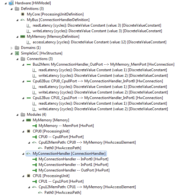
As described in the beginning of this section, a single data access may result in a series of events. Expected simulation behavior is as follows: When the discrete-event simulator encounters a runnable item for a data read access at CPU0, we add an event for one tick later to the event queue of the simulator, denoting passing the connection from CPU0 to the connection handler MyConnectionHandler. (For simplicity, we do not use time durations calculated from the CPU0's frequency here, what would be required to determine the correct point in simulated time for the event). After passing the connection, the state of MyConnectionHandler is relevant for the next event: Either MyConnectionHandler is occupied by a data access (from CPU1), a data access arrives at the same time, or MyConnectionHandler is available.
- If MyConnectionHandler is available, we add an event for three ticks later-this is the read latency of the connection handler.
- If a data access from CPU1 arrives at the same time, the connection handler handles this data access based on the selected arbitration mechanism (attribute not shown in the screen shot – we assume priority based with a higher priority for CPU1). We add an event for three ticks later, when MyConnectionHandler is available again. We then check again for data accesses from CPU1 at the same time and set a corresponding event.
- If MyConnectionHandler is occupied, we add an event for whenever the connection handler is not occupied anymore. We then check for data accesses from CPU1 at the same time and set a corresponding event.
Eventually, MyConnectionHandler may handle the read access from CPU0, and when the simulator reacts on the corresponding event, we add an event for one tick later, as this is the read latency for the connection between the connection handler and the memory. The final event for this read data access from CPU0 results from the access latency of the memory (twelve ticks). When the simulator reacts on that final event, the read access from CPU0 is completed and the simulator can handle the next runnable item at CPU0, if available.
Note that in the above example there is only one contention point. We thus could reduce the number of events for an optimized simulation. Further, note that we ignore size of data elements in this example. We could use
data rates instead of latencies at connections, the connection handler, and the memory to respect data sizes in timing simulation or work with the bit width of ports. Furthermore beside constant latency values it is also possible to use distributions, in this case the simulator role the dice regarding the distribution. At a last note, adding to the discussion of different detail levels: Depending on use-case, modeling purpose, and timing analysis tool, there may be best practice defined for modeling. For instance, one tool may rely on data rates, while other tools require latencies but only at memories and connection handlers, not connections. Tool specific model transformations and validation rules should handle and define such restrictions.
Structural Modeling of Heterogeneous Platforms
To master the rising demands of performance and power efficiency, hardware becomes more and more diverse with a wide spectrum of different cores and hardware accelerators. On the computation front, there is an emergence of specialized processing units that are designed to boost a specific kind of algorithm, like a cryptographic algorithm, or a specific math operation like "multiply and accumulate". As one result, the benefit of a given function from hardware units specialized in different kinds may lead to nonlinear effects between processing units in terms of execution performance of the algorithm: while one function may be processed twice as fast when changing the processing unit, another function may have no benefit at all from the same change. Furthermore the memory hierarchy in modern embedded microprocessor architectures becomes more complex due to multiple levels of caches, cache coherency support, and the extended use of DRAM. In addition to crossbars, modern SoCs connect different clusters of potentially different hardware components via a Network on Chip. Additionally, power and frequency scaling is supported by state of the art SoCs. All these characteristics of modern and performant SoCs (specialized processing units, complex memory hierarchy, network like interconnects and power and frequency scaling) were only partially supported by the former Amalthea hardware model. Therefore, to create models of modern heterogeneous systems, new concepts of representing hardware components in a flexible and easy way are necessary: Our approach supports modeling of manifold hierarchical structures and also domains for power and frequencies. Furthermore, explicit cache modules are available and the possibilities for modeling the whole memory subsystem are extended, the connection between hardware components can be modeled over different abstraction layers. Only with such an extended modeling approach, a more accurate estimation of the system performance of state of the art SoCs becomes feasible.
Our intention is allowing to create a hardware model once at the beginning of a development process. Ideally, the hardware model will be provided by the vendor. All performance relevant attributes regarding the different features of hardware components like a floating point unit or how hardware components are interconnected should be explicitly represented in the model. The main challenge for a hardware/software performance model is then to determine certain costs, e.g. the net execution time of a software functionality mapped to a processing unit. Costs such as execution time, in contrast to the hardware structure, may change during development time – either because the implementation details evolve from initial guess to real-world measurements, the implementation is changed, or the tooling is changed. Therefore, the inherent attributes of the hardware, e.g. latency of an access path, should be decoupled from the mapping or implementation dependent costs of executing functions. We know from experience that it is necessary to refine these costs constantly in the development process to increase accuracy of performance estimation. Refinement denotes incorporation of increasing knowledge about the system. Therefore, such a refinement should be possible in an efficient way and also support re-use of the hardware model. The corresponding concepts are detailed in the following section.
Recipe and Feature concept: An outlook of an upcoming approach
Disclaimer: Please note that the following describes work in progress – what we call "recipes" later is not yet part of the meta-model, and the concept of "features" is not final.
The main driver of the concept described here is separation of implementation dependent details from structural or somehow "solid" information about a hardware/software system. This follows the separation of concerns paradigm, mainly to reduce refinement effort, and foster model re-use: As knowledge about a system grows during development, e.g. by implementing or optimizing functionality as software, the system model should be updated and refined efficiently, while inherent details shall be kept constant and not modified depending on the implementation.
An example should clarify this approach: For timing simulation, we require the net execution time of a software function executed on the processing unit it is mapped onto. This cost of the execution depends on the implementation of the algorithm, for instance, as C++ code, and the tool chain producing the binary code that eventually is executed. In that sense, the
execution needs of the algorithm (for instance, a certain number of "multiply and accumulate" operations for a matrix operation) are naturally fixed, as well as the
features provided by the processing unit (for instance, a dedicated MAC unit requiring one tick for one operation, and a generic integer unit requiring 0.5 ticks per operation). However is implementation- and tool-chain-dependent how the actual execution needs of the algorithm are served by the execution units. Without changing the algorithm or the hardware, optimization of the implementation may make better use of the hardware, resulting in reduced execution time. The above naturally draws the lines for our modeling approach: Execution needs (on an algorithmic level) are inherent, as well as features of the hardware. Keeping these information constant in the model is the key for re-use; implementation dependent change of costs, such as lower execution time by an optimized implementation in C++ or better compiler options, change during development and are modeled as
recipe. A "recipe" thus takes execution needs of software and features of the hardware as input and results in costs, such as the net execution time. Consequently, recipes are the main area of model refinement during development. The concept is illustrated below.
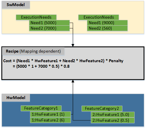
Note that flexibility is part of the design of this approach. Execution needs and features are not limited to a given set, and recipes can be almost arbitrary prescripts of computation. This allows to introduce new execution needs when required to favorable detail an algorithm. For instance, the execution need "convolution-VGG16" can be introduced to model a specific need for a deep learning algorithm. The feature "MAC" of the executing processing unit provides costs in ticks corresponding to perform a MAC operation. The recipe valid for the mapping then uses these two attributes to compute the net execution time of "convolution-VGG16" in ticks, for instance, by multiplying the costs of xyz MAC operations with a penalty factor of 0.8. Note that with this approach execution needs may be translated very differently into costs, using different features.
To further motivate this approach, we give some more benefits and examples of beneficial use of the model:
- Given execution needs of a software function that directly correspond the features of processing units, the optimal execution time may be computed (peak performance).
- While net execution time is the prime example of execution needs, features, and recipes, the concept is not limited to "net execution time recipes", recipes for other performance numbers such as power consumption are possible.
- Recipes can be attached at different "levels" in the model: At a processing unit and at a mapping. If present, the recipe at mapping level has precedence.
General Hardware Model Overview
The design of the new hardware model is focusing on flexibility and variety to cover different kind of designs to cope with future extensions, and also to support different levels of abstraction. To reduce the complexity of the meta model for representing modern hardware architectures, as less elements as possible are introduced. For example, dependent of the abstraction level, a component called
ConnectionHandler can express different kind of connection elements, e.g. a crossbar within a SoC or a CAN bus within an E/E-architecture. A simplified overview of the meta model to specify hardware as a model is shown below. The components
ConnectionHandler, ProcessingUnit, Memory and
Cache are referred in the following as basic components.
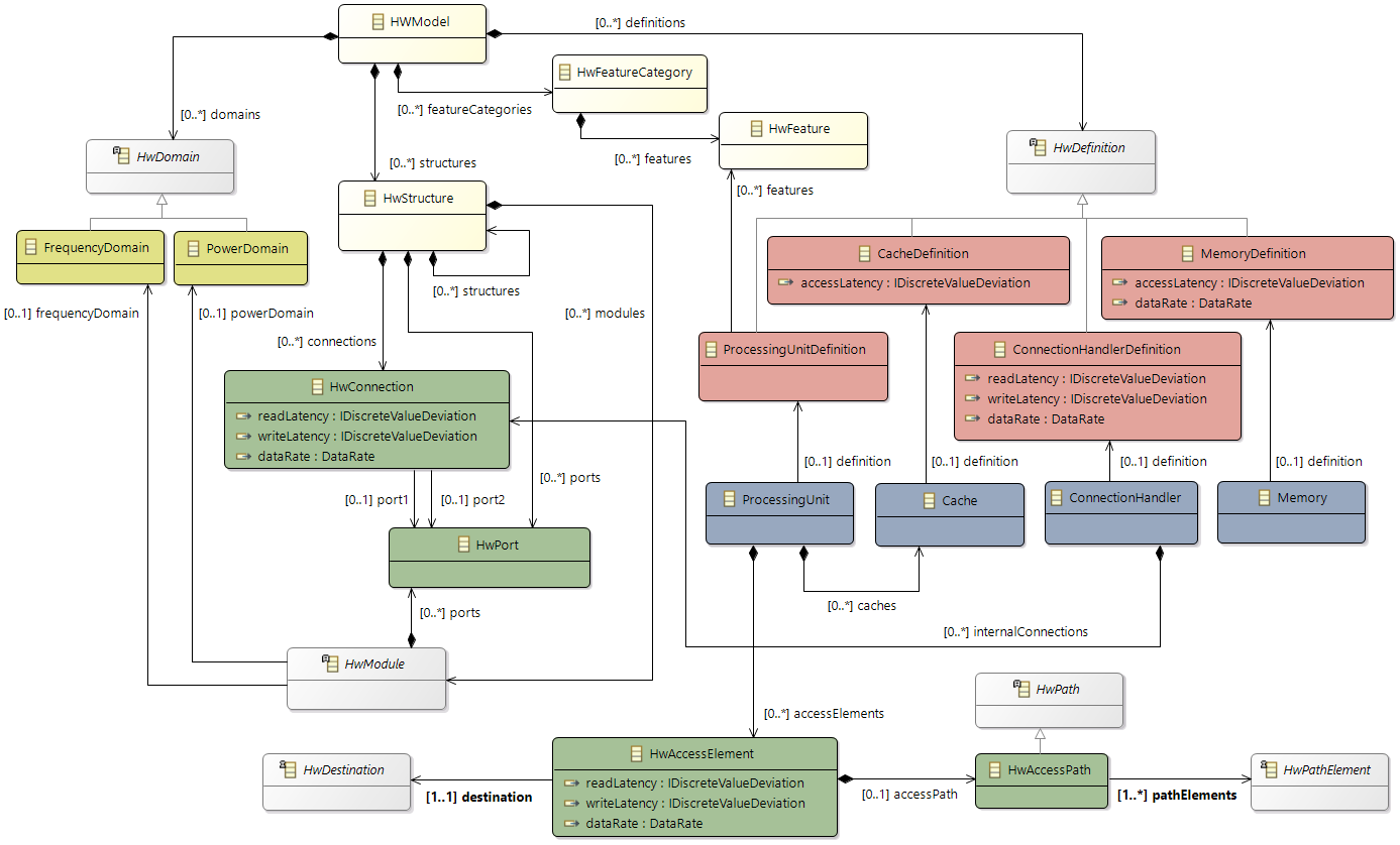
Class diagram of the hardware model
The root element of a hardware model is always the
HwModel class that contains all domains (power and frequency), definitions, and hardware features of the different component definitions. The hierarchy within the model is represented by the
HwStructure class, with the ability to contain further
HwStructure elements. Therewith arbitrary levels of hierarchy could be expressed. Red and blue classes in the figure are the definitions and the main components of a system like a memory or a core.
The next figure shows the modeling of a processor. The
ProcessingUnitDefiniton, which is created once, specifies a processing unit with general information (which can be a CPU, GPU, DSP or any kind of hardware accelerator). Using a definition that may be re-used supports quick modeling for multiple homogeneous components within a heterogeneous architecture.
ProcessingUnits then represent the physical instances in the hardware model, referencing the
ProcessingUnitDefiniton for generic information, supplemented only with instance specific information like the
FrequencyDomain.
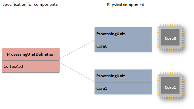
Link between definitions and module instances (physical components)
Yellow represents the power and frequency domains that are always created at the top level of the hardware model. It is possible to model different frequency or voltage values, e.g., when it is possible to set a systems into a power safe mode. All components that reference the domain are then supplied with the corresponding value of the domain.
All the green elements in the figure are related to communication (together with the blue base component
ConnectionHandler). Green modeling elements represent ports, static connections, and the access elements for the
ProcessingUnits. These
ProcessingUnits are the master modules in the hardware model. The following example shows two
ProcessingUnits that are connected via a
ConnectionHandler to a
Memory. There are two different possibilities to specify the access paths for
ProcessingUnits like it is shown for ProcessingUnit_2 in the next figure. Every time a
HwAccessElement is necessary to assign the destination e.g. a
Memory component. This
HwAccessElement can contain a latency or a data rate dependent on the use case. The second possibility is to create a
HwAccessPath within the
HwAccessElement which describes the detailed path to the destination by referencing all the
HwConnections and
ConnectionHandlers. It is even possible to reference a cache component within the
HwAccessPath to express if the access is cached or non-cached. Furthermore it is possible to set addresses for these
HwAccessPath to represent the whole address space of a
ProcessingUnit. A typical approach would be starting with just latency or data rates for the communication between components and enhance the model over time to by switching to the
HwAccessPaths.
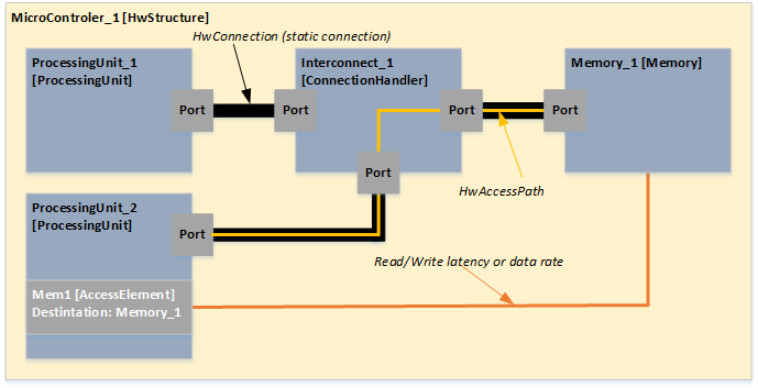
Access elements in the hardware model
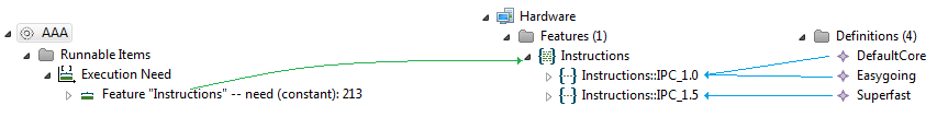
Current implementation with features and the connection to the SW Model
In the previous chapter the long time goal of the feature and recipe concept is explained. As an intermediate step before introducing the recipes we decided to connect the HwModel and SwModel by referencing to the name of the hardware
FeatureCategories from the
ExecutionNeed element in a Runnable. The following figure shows this connection between the grey Runnable item block and the white Features block. Due to the mapping (Task or Runnable to ProcessingUnit) the corresponding feature value can be extracted out of the ProcessingUnitDefinition.
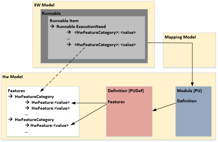
An example based on the old hardware model is the "instruction per cycle" value (IPC). To model an IPC with the new approach a
HwFeatureCategory is created with the name
Instructions. Inside this category multiple IPC values can be created for different
ProcessingUnitDefinitions.
Note: In version 0.9.0 to 0.9.2 exists a default ExecutionNeed Instructions together with a the HwFeatre IPC the cycles can be calculated by dividing the Instructions by the IPC value.
Execution needs example
Interpretation of latencies in the model
In the model read and write access latencies are used. An alternative which is usually used in specifications or by measurements are request and response latencies. The following figure shows a typical communication between two components. The interpretation of a read and write latency for example at
ConnectionHandlers is the following:
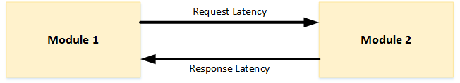
-
readLatency = requestLatency + response Latency
-
writeLatency = requestLatency
The access latency of a
Memory component is always added to the read or write latency from the communication elements, independent if its one latency from an
HwAccessElement or multiple latencies from a
HwAccessPath.
As example in case of using only read and write latencies:
-
totalReadLatency = readLatency (HwAccessElement) + accessLatency (Memory)
-
totalWriteLatency = writeLatency (HwAccessElement) + accessLatency (Memory)
An example in case of using an access element with a hardware access path:
n = Number of path elements
-
totalReadLatency = Sum 1..n ( readLatency(p) ) + accessLatency (Memory)
-
totalWriteLatency = Sum 1..n ( writeLatency(p) ) + accessLatency (Memory)
PathElements could be
Caches,
ConnectionHandlers and
HwConnections. In very special cases also a
ProcessingUnit can be a
PathElement the
ProcessingUnit has no direct effect on the latency. In case the user want to express a latency it has to be annotated as
HwFeature.
2.2.3 Software (development)
The AMALTHEA System Model can also be used in early phases of the development process when only limited information about the resulting software is available.
Runnables
The
Runnable element is the basic software unit that defines the behavior of the software in terms of runtime and communication. It can be described on different levels of abstraction:
- timing only (activation and runtime)
- including communication (in general)
- adding detailed activity graphs
To allow a more detailed simulation a description can also include statistical values like deviations or probabilities. This requires additional information that is typically derived from an already implemented function. The modeling of observed behavior is described in more detail in chapter
Software (runtime).
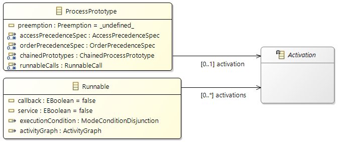
Process Prototypes
Process Prototypes are used to define the basic data of a task. This is another possibility to describe that a set of Runnables has a similar characteristic (e.g. they have the same periodic activation).
A prototype can then be processed and checked by different algorithms. Finally a partitioning algorithm generates (one or more) tasks that are the runtime equivalents of the prototype.
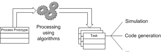
This processing can be guided by specifications that are provided by the function developers:
- The
Order Specification is a predefined execution order that has to be guaranteed.
- An
Access Specification defines exceptions from the standard write-before-read semantics.
Constraints
In addition the partitioning and mapping can be restricted by
Affinity Constraints that enforce the pairing or separation of software elements and by
Property Constraints that connect hardware capabilities and the corresponding software requirements.
The
Timing Constraints will typically be used to check if the resulting system fulfills all the requirements.
Activations
Activations are used to specify the intended activation behavior of
Runnables and
ProcessPrototypes. Typically they are defined before the creation of tasks (and the runnable to task mappings). So this is a way to cluster runnables and to document when the runnables should be executed.
The following activation patterns can be distinguished:
- Single: single activation
- Periodic: periodic activation with a specific frequency
- Sporadic: recurring activation without following a specific pattern
- Event: activation triggered by a
TriggerEvent
- Custom: custom activation (free textual description)
To describe a specific (observed) behavior at runtime there are
Stimuli in the AMALTHEA model. They can be created based on the information of the specified activations.
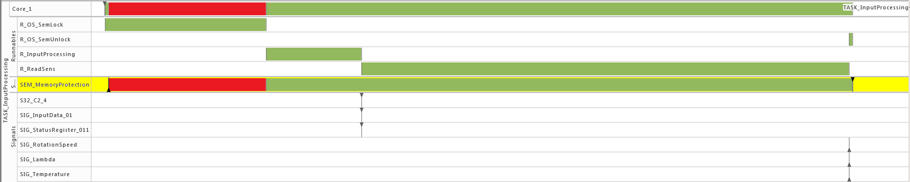
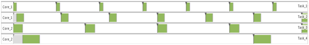
2.2.4 Software (runtime)
During runtime, the dynamic behavior of the software can be observed. The following Gantt chart shows an excerpt of such a dynamic behavior.
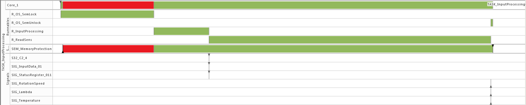
To model the observed behavior in the AMALTHEA model there are schedulable units (Processes) that contain the basic software units (Runnables) and stimuli that describe when the processes are executed. Statistical elements like distributions (Gauss, Weibull, ...) are also available in the model. They allow describing the variation of values if there are multiple occurrences.
In the following sections, a high level description of the individual elements of a software description that define the dynamic behavior are presented.
Processes (Tasks or ISRs)
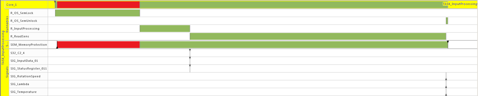
Processes represent executable units that are managed by an operating system scheduler. A process is thus the smallest schedulable unit managed by the operating system. Each process also has its own name space and resources (including memory) protected against use from other processes. In general, two different kinds of processes can be distinguished: task and Interrupt Service Routine (ISR). Latter is a software routine called in case of an interrupt. ISRs have normally higher priority than tasks and can only be suspended by another ISR which presents a higher priority than the one running. In the Gantt chart above, a task called 'TASK_InputProcessing' can be seen. All elements that run within the context of a process are described in the following sections.
Runnables
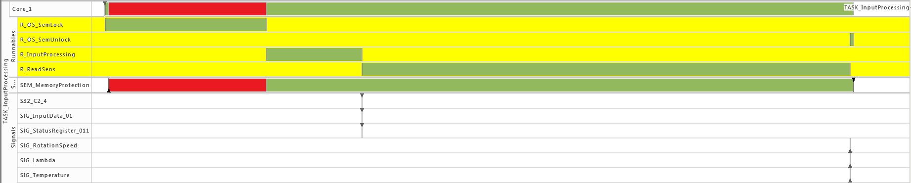
Runnables are basic software units. In general it can be said that a Runnable is comparable to a function. It runs within the context of a process and is described by a sequence of instructions. Those instructions can again represent different actions that define the dynamic behavior of the software. Following, such possible actions are listed:
- Semaphore Access: request/release of a semaphore
- Label Access: reading/writing a data signal
- Ticks: number of ticks (cycles) to be executed
- ...
In the following sections elements, that can be of concern within a runnable, are described in more detail.
Labels
Labels represent the system's view of data exchange. As a consequence, labels are used to represent communication in a flattened structure, with (at least) one label defined for each data element sent or received by a Runnable instance.
Semaphore
The main functionality of a semaphore is to control simultaneous use of a single resource by several entities, e.g. scheduling of requests, multiple access protection.
Stimulation
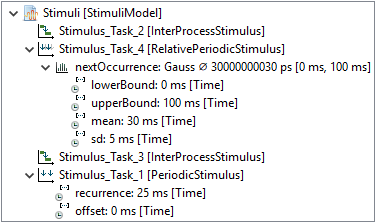
Before, we described the dynamic behavior of a specific process instance. In general however, a process is not only activated once but many times. The action of activating a process is called stimulation. The following stimulation patterns are typically used for specification:
- Single: single activation of a process
- Periodic: periodic activation of a process with a specific frequency
- VariableRate: periodic activations based on other events, like rotation speed
- Event: activation triggered by a
TriggerEvent
- InterProcess: activations based on an explicit inter-process trigger
2.2.5 General Concepts
Grouping of elements (Tags, Tag groups)
It is possible to use
Tags for grouping elements of the model.
Custom Properties
The AMALTHEA model provides
Custom Properties to enhance the model in a generic way. These can be used for different kind of purpose:
- Store attributes, which are relevant for your model, but not yet available at the elements
- Processing information of algorithms can be stored in that way, e.g. to mark an element as already processed
Support of Packages
In Amalthea model
(from APP4MC 0.9.7 version) there is a feature to support grouping of following model elements listed below in a package:
- Component
- Composite
- MainInterface
Above mentioned classes are implementing interface
IComponentStructureMember
ComponentStructure element in Amalthea model represents a package, and this can be referred by above mentioned elements.
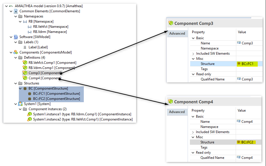
Example of using Package
Amalthea model contains a parent ComponentStructure "BC" and two child ComponentStructure's "FC1", "FC2".
- Component element "Comp3" is associated to ComponentStructure "FC1" and the Component element "Comp4" is associated to ComponentStructure "FC2"
This representation demonstrates the grouping of the elements into different packages.
Support of Namespaces
In Amalthea model
(from APP4MC 0.9.7 version) there is a feature to have Namespace for the following model elements (
which are implementing interface
INamespaceMember
):
- BaseTypeDefinition
- Channel
- Component
- Composite
- DataTypeDefinition
- Label
- MainInterface
- Runnable
- TypeDefinition
Advantage of having Namespace is, there can be multiple elements defined with the same name but with different Namespace
(this feature will also be helpful to support c++ source code generation ). If Namspace is specified in Amalthea model for a specific model element, then its unique name is built by considering the "Namespace text + name of the element"
Example of using Namespace
As shown in the below screenshot, there are two Component elements with the name "Comp1" but referring to different Namespace objects, which is making them unique. In this case, display in the UI editor is also updated by showing the Namespace in the prefix for the Amalthea element name.
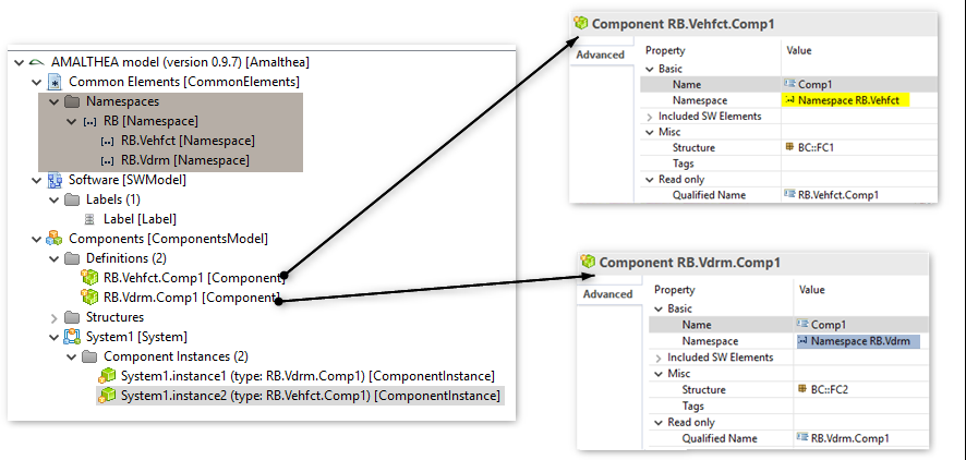
Below is the text representation of the Amalthea model which shows the ComponentInstance elements referring to different Component elements. As mentioned above, highlighted text shows that unique name of the Component element
__ is used all the places where it is referenced __(to make it unique)

Additional Information:
- As soon as Namespace elements are used in Amalthea model, AMXMI file is updated with additional attribute xmi:id for all elements implementing IReferable interface.
- On Amalthea model element implementing INamed interface, in addition to getName() API, getQualifiedName() API is available which returns <namespace string value>.getName()
2.2.6 Scheduling
Scheduler to Core assignment
We distinguish between physical mapping and responsibility
-
Executing Core means a scheduler produces algorithmic overhead on a core
-
Responsibility means a scheduler controls the scheduling on core(s)
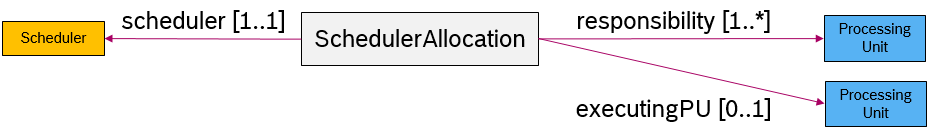
Task to Scheduler assignment
Tasks have a core affinity and are assigned to a scheduler
-
Core Affinity Specifies the possible cores the task can run on. If only one core is specified, the task runs on this core. If multiple cores are specified, the task can migrate between the cores.
-
Scheduler specifies the unique allocation of the task to a scheduler.
The scheduling parameters are determined by the scheduling algorithm and are only valid for this specific task – scheduler combination. Therefore the parameters are specified in the TaskAllocation object.

Scheduler hierarchies
Schedulers can be arranged in a hierarchy via SchedulerAssociations. If set, the parent scheduler takes the initial decision and delegates to a child-scheduler. If the child-scheduler is a reservation based server, it can only delegate scheduling decisions to its child scheduler. If it is not a server, it can take scheduling decisions.
The scheduling parameters for the parent scheduler are specified in the SchedulerAssociation, just as it would have for task allocations.
If a reservation based server has only one child (this can either be a process or a child scheduler), the scheduling parameters specified in this single child allocation will also be passed to the parent scheduler. The example below shows this for the EDF scheduler on the right hand side.

2.2.7 Communication via channels
Channel
Sender and receiver communicating via a channel by issuing send and receive operations; read policy and transmission policy define communication details.
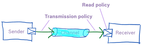
A channel is specified by three attributes:
-
elementType: the type that is sent to or read from the channel.
-
defaultElements: number of elements initially in the channel (at start-up).
-
maxElements (integer) denoting a buffer limit, that is, the channel depth. In other words, no more than maxElements elements of the given element type may be stored in the channel.
Channel Access
In the basic thinking model, all elements are stored as a sequential collection in the channel.
Sending
A runnable may send elements to a channel by issuing send operations.
The send operation has a single parameter:
-
elements (integer): Number of elements that are written.
Receiving
A runnable may receive elements from a channel by issuing receive operations.
The receive operation is specified with a
receive policy that defines the main behaviour of the operation:
-
LIFO (last-in, first-out) is chosen if processing the last written elements is the primary focus and thereby missing elements is tolerable.
-
FIFO (first-in, first-out) is chosen if every written element needs to be handled, that is, loss of elements is not tolerable.
-
Read will received elements without modifying the channel
-
Take will remove the received elements from the channel
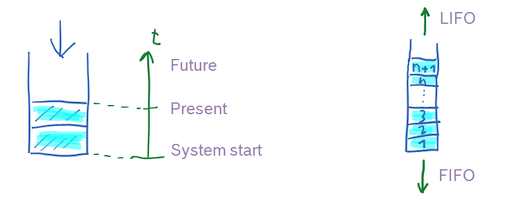
The receive policy defines the direction a receive operation takes effect with LIFO accesses are from top of the sequential collection, while with FIFO accesses are from bottom of the sequential collection-and they define if the receive operation is destructive (take) or non-destructive) read.
Each operation further has two parameters and two attributes specifying the exact behavior. The two parameters are:
-
elements (integer): Maximum number n of elements that are received.
-
elementIndex (integer): Position (index i) in channel at which the operation is effective. Zero is the default and denotes the oldest (FIFO) or newest element (LIFO) in the channel.
In the following several examples are shown, of how to read or take elements out of a channel with the introduced parameters.
Two attributes further detail the receive operation:
-
lowerBound (integer): Specify the minimum number of elements returned by the operation. The value must be in the range [0,n], with n is the value of the parameter elements. Default value is n.
-
dataMustBeNew (Boolean): Specify if the operation must only return elements that are not previously read by this Runnable. Default value is false.
Transmission Policy
To further specify how elements are accessed by a runnable in terms of computing time, an optional transmission policy may specify details for each receive and send operation. The intention of the transmission policy is to reflect computing demand (time) depending on data.
The transmission policy consists of the following attributes:
-
chunkSize: Size of a part of an element, maximum is the element size.
-
chunkProcessingTicks (integer): Number of ticks that will be executed to process one chunk (algorithmic overhead).
-
transmitRatio (float): Specify the ratio of each element that is actually transmitted by the runnable in percent. Value must be between [0, 1], default value is 1.0.
Example for using transmission policy to detail the receiving phase of a runnable execution. Two elements are received, leading to transmission time as given in the formula. After the receiving phase, the runnable starts with the computing phase.
2.2.8 Data Dependencies
Overview
It is possible to specify potential data dependencies for written data. More specifically, it is now possible to annotate at write accesses what other data potentially have influenced the written data. A typical "influence" would be usage of data for computing a written value. As such data often comes from parameters when calling a runnable, it is now also possible to specify runnable parameters in Amalthea and their potential influence on written data.
Semantics of the new attributes in Amalthea is described in detail below. In general, these data dependency extensions are considered as a way to explicitly model details that help for visualization or expert reviews. For use cases such as timing simulation the data dependency extensions are of no importance and should be ignored.
Internal Dataflow
In Embedded Systems, external dataflow is specified with reads and writes to labels, which are visible globally. This is sufficient for describing the inter-runnable communication and other use-cases like memory optimization. Nevertheless, for description of signal flows along an event chain, it is also necessary to specify the internal dataflow so that the connection between the read labels and the written labels in made.
Internal dataflow is specified as dependency of label writes to other labels, parameters of the runnable or event return values of called runnables. With this information, the connection of reads to writes of label can be drawn.
The internal dependencies are typically generated through source code analysis. The analysis parses the code and determines all writes to labels. For each of those positions, a backward slicing is made on the abstract syntax tree to derive all reads that influence this write. This collection is then stored as dependency at the write access.
Based upon this data a developer can now track a signal flow along from the sensor over several other runnables to the actuator. Existing event-chains can be automatically validated to contain a valid flow by checking if the segments containing a read label event and write label event within the same runnable are connected by an internal dependency. Without internal dependencies, this would introduce a huge manual effort. Afterwards the event-chains can be simulated and their end-to-end latencies determined with the usual tools.
2.2.9 Memory Sections
Purpose
Memory Sections are used for the division of the memory (RAM/ROM) into different blocks and allocate the "software" memory elements (
e.g. Labels), code accordingly inside them.
Each Memory Section has certain specific properties (
e.g. faster access of the elements, storing constant values). By default compiler vendors provide certain Memory Sections (
e.g. .data, .text) and additional Memory Sections can be created based on the project need by enhancing the linker configuration.
Definition
A "Memory Section" is a region in memory (RAM/ROM) and is addressed with a specific name. There can exist multiple "Memory Sections" inside the same Memory (RAM/ROM) but with different names. Memory Section names should be unique across the Memory (RAM/ROM).
Memory Sections can be of two types:
- Virtual Memory Section
- Physical Memory Section
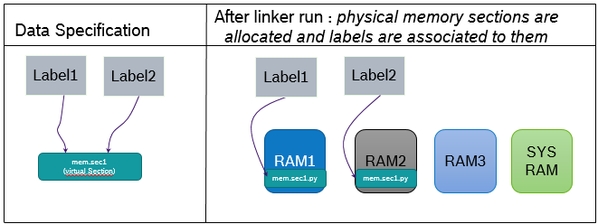
Virtual Memory Section
"Virtual Memory Sections" are defined as a part of data specification and are associated to the corresponding Memory Elements (e.g. Label's) during the development phase of the software. Intention behind associating "Virtual Memory Sections" to Memory elements like Label's is to control their allocation in specific Memory (e.g. Ram1 or Ram2) by linker.
As a part of linker configuration – It is possible to specify if a "Virtual Memory Section"
(e.g. mem.Sec1) can be part of certain Memory
(e.g. Ram1/Ram2/SYSRAM but not Ram3).
Example:
Software should be built for ManyCore ECU – containing 3 Cores
(Core1, Core2, Core3). Following RAMs are associated to the Cores: Ram1 – Core1, Ram2 – Core2, Ram3 – Core3, and also there is SYSRAM.
Virtual Memory Section : mem.sec1
(is defined as part of data specification) is associated to Label1 and Label2.
In Linker configuration it is specified that mem.sec1 can be allocated only in Ram1 or Ram2.
Below diagram represents the
linker configuration content
- w.r.t. possibility for physical allocation of mem.sec1 in various memories .
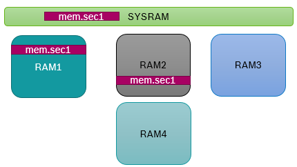
Based on the above configuration – Linker will allocate Label1, Label2 either in Ram1/Ram2/SYSRAM but not in Ram3/Ram4.
Physical Memory Section
"Physical Memory Sections" are generated by linker. The linker allocates various memory elements (e.g. Label's) inside "Physical Memory Sections".
Each "Physical Memory Section" has following properties:
- Name – It will be unique across each Memory
- Start and End address – This represents the size of "Physical Memory Section"
- Associated Physical Memory
(e.g. Ram1 or Ram2)
Example:
There can exist mem.sec1.py inside Ram1 and also in Ram2. But these are physically two different elements as they are associated to different memories (Ram1 and Ram2) and also they have different "start and end address".
Below diagram represents the information w.r.t. virtual memory sections
(defined in data specification and associated to memory elements) and physical memory sections
(generated after linker run).
Modeling Memory Section information in AMALTHEA
- As described in the above concept section:
- Virtual memory sections are used:
- To specify constraints for creation of Physical memory sections by linker
- To control allocation of data elements (e.g. Labels) in a specific memory
(e.g. Ram1/Ram2/SYSRAM)
- Physical memory sections are containing the data elements after linker run
(representing the software to be flashed into ECU)
Below figure represents the modeling of "Memory Section" (both virtual and physical) information in AMALTHEA model:
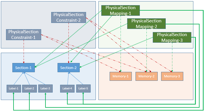
Below are equivalent elements of AMALTHEA model used for modeling the Memory Section information:
-
Section
- This element is equivalent to Virtual Memory Section defined during the SW development phase.
- As a part of data specification defined in the sw-development phase, a Section object
(with specific name) is associated to Label and Runnable elements.
-
PhysicalSectionConstraint
- This element is equivalent to the constraint specified in the linker configuration file, which is used to instruct linker for the allocation of Physical Memory Sections in specified Memories.
- PhysicalSectionContraint is used to specify the combination of Virtual Memory Section and Memories
(which can be considered by linker for generation of Physical Memory Sections).
Example:
PhysicalSectionConstraint-1 is specifying following relation "Section-1" <--> "Memory-1", "Memory-2". This means that the corresponding Physical Memory Section for "Section-1" can be generated by linker in "Memory-1" or in "Memory-2" or in both.
-
PhysicalSectionMapping
- This element is equivalent to Physical Memory Section generated during the linker run.
- Each PhysicalSectionMapping element:
- Contains the Virtual Memory Section
(e.g. Section-1) which is the source.
- is associated to a specific Memory and it contains the start and end memory address
(difference of start and end address represents the size of Physical Memory Section).
- contains the data elements
(i.e. Labels, Runnables part of the final software).
Note: There is also a possibility to associate multiple Virtual Memory Section's as linker has a concept of grouping Virtual Memory Sections while generation of Physical Memory Section.
Example:
For the same Virtual Memory Section
(e.g. Section-1), linker can generate multiple Physical Memory Sections in different Memories
(e.g. PhysicalSectionMapping-1, PhysicalSectionMapping-2). Each PhysicalSectionMapping element is an individual entity as it has a separate start and end memory address.
2.3 Examples
2.3.1 Modeling Example 1
General information
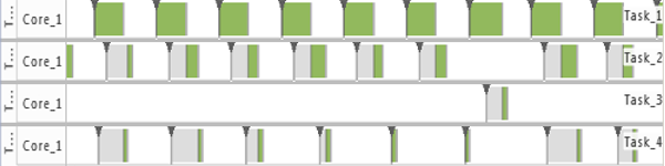
Modeling Example 1 describes a simple system consisting of 4 Tasks, which is running on a dual core processor.
The following figure shows the execution footprint in a Gantt chart:
In the following sections, the individual parts of the AMALTHEA model for Modeling Example 1 are presented followed by a short description of its elements.
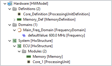
Hardware Model
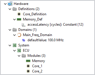
The hardware model of Modeling Example 1 consists as already mentioned of a dual core processor.
The following gives a structural overview on the modeled elements.
There, the two cores, 'Core_1' and 'Core_2', have a static processing frequency of 100 MHz each, which is specified by the corresponding quartz oscillator 'Quartz'.
Operating System Model
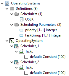
The operating system (OS) model defines in case of Modeling Example 1 only the needed Scheduler.
Since a dual core processor has to be managed, two schedulers are modeled correspondingly.
In addition to the scheduler definition used by the scheduler, in this case OSEK, a delay of 100 ticks is set, which represents the presumed time the scheduler needs for context switches.
| Scheduler |
Type |
Algorithm |
Delay |
|
Scheduler_1
|
Constant |
OSEK |
100 ticks |
|
Scheduler_2
|
Constant |
OSEK |
100 ticks |
Mapping Model
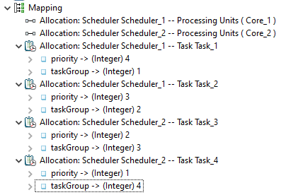
The mapping model defines allocations between different model parts.
On the one hand, this is the allocation of processes to a scheduler. In case of Example 1, 'Task_1' and 'Task_2' are managed by 'Scheduler_1', while the other tasks are managed by 'Scheduler_2'. Scheduler specific parameters are set here, too. For the OSEK scheduler these are 'priority' and 'taskGroup'. Each task has a priority assigned according its deadline, meaning the one with the shortest deadline, 'Task_1', has the highest priority, and so on.
On the other hand the allocation of cores to a scheduler is set. For Modeling Example 1 two local schedulers were modeled. As a consequence, each scheduler manages one of the processing cores.
A comprehension of the modeled properties can be found in the following tables:
Executable Allocation with Scheduling Parameters
| Scheduler |
Process |
priority |
taskGroup |
| Scheduler_1 |
Task_1 |
4 |
1 |
| Scheduler_1 |
Task_2 |
3 |
2 |
| Scheduler_2 |
Task_3 |
2 |
3 |
| Scheduler_2 |
Task_4 |
1 |
4 |
Core Allocation
| Scheduler |
Core |
| Scheduler_1 |
Core_1 |
| Scheduler_2 |
Core_2 |
Software Model
Tasks
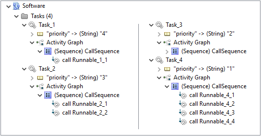
As already mentioned above, the software model of Modeling Example 1 consists exactly of four tasks, named 'Task_1' to 'Task_4'. Each task is preemptive and also calls a definitive number of Runnables in a sequential order.
A comprehension of the modeled properties can be found in the following table:
| Task |
Preemption |
MTA* |
Deadline |
Calls |
|
Task_1
|
Preemptive |
1 |
75 ms |
1) Runnable_1_1 |
|
Task_2
|
Preemptive |
1 |
115 ms |
1) Runnable_2_1 |
| 2) Runnable_2_2 |
|
Task_3
|
Preemptive |
1 |
300 ms |
1) Runnable_3_1 |
| 2) Runnable_3_2 |
| 3) Runnable_3_3 |
|
Task_4
|
Preemptive |
1 |
960 ms |
1) Runnable_4_1 |
| 2) Runnable_4_2 |
| 3) Runnable_4_3 |
| 4) Runnable_4_4 |
*MTA = Multiple Task Activation Limit
Runnables
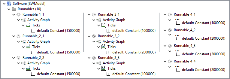
In addition to the task, the software model also contains a definition of Runnables.
For Modeling Example 1, ten individual Runnables are defined.
The only function of those in this example is to consume processing resources.
Therefore, for each Runnable a constant number of instruction cycles is stated.
A comprehension of the modeled properties can be found in the following table:
| Runnable |
InstructionCycles |
| Runnable_1_1 |
1500000 |
| Runnable_2_1 |
1500000 |
| Runnable_2_2 |
1500000 |
| Runnable_3_1 |
1000000 |
| Runnable_3_2 |
2000000 |
| Runnable_3_3 |
1000000 |
| Runnable_4_1 |
1000000 |
| Runnable_4_2 |
2000000 |
| Runnable_4_3 |
3000000 |
| Runnable_4_4 |
2000000 |
Stimuli Model
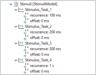
The stimulation model defines the activations of tasks.
Since the four tasks of Modeling Example 1 are activated periodically, four stimuli according their recurrence are modeled.
A comprehension of the modeled properties can be found in the following table:
| Stimulus |
Type |
Offset |
Recurrence |
| Stimulus_Task_1 |
Periodic |
0 ms |
180 ms |
| Stimulus_Task_2 |
Periodic |
0 ms |
200 ms |
| Stimulus_Task_3 |
Periodic |
0 ms |
300 ms |
| Stimulus_Task_4 |
Periodic |
0 ms |
1 s |
2.3.2 Modeling Example 2
General information
Modeling Example 2 describes a simple system consisting of 4 Tasks, which is running on a single core processor.
The following figure shows the execution footprint in a Gantt chart:
In the following sections, the individual parts of the AMALTHEA model for Modeling Example 2 are presented followed by a short description of its elements.
Hardware Model
The hardware model of Modeling Example 2 consists as already mentioned of a single core processor.
The following gives a structural overview on the modeled elements.
There, the core, 'Core_1' , has a static processing frequency of 600 MHz each, which is specified by the corresponding quartz oscillator 'Quartz_1'.
Operating System Model
The operating system (OS) model defines in case of Modeling Example 2 only the needed Scheduler.
Since only a single core has to be managed, a single scheduler is modeled correspondingly.
In addition to the scheduler definition used by the scheduler, in this case OSEK, a delay of 100 ticks is set, which represents the presumed time the scheduler needs for context switches.
| Scheduler |
Type |
Algorithm |
Delay |
|
Scheduler_1
|
Constant |
OSEK |
100 ticks |
Mapping Model
The mapping model defines allocations between different model parts.
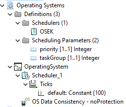
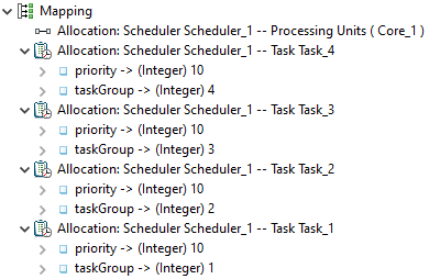
On the one hand, this is the allocation of processes to a scheduler. Since there is only one scheduler available in the system, all four tasks are mapped to 'Scheduler_1'. Scheduler specific parameters are set here, too. For the OSEK scheduler these are 'priority' and 'taskGroup'. All tasks have assigned the same priority (10) to get a cooperative scheduling.
On the other hand the allocation of cores to a scheduler is set. As a consequence, the scheduler manages the only available processing core.
A comprehension of the modeled properties can be found in the following tables:
Executable Allocation with Scheduling Parameters
| Scheduler |
Process |
priority |
taskGroup |
| Scheduler_1 |
Task_1 |
10 |
1 |
| Scheduler_1 |
Task_2 |
10 |
2 |
| Scheduler_1 |
Task_3 |
10 |
3 |
| Scheduler_1 |
Task_4 |
10 |
4 |
Core Allocation
| Scheduler |
Core |
| Scheduler_1 |
Core_1 |
Software Model
Tasks
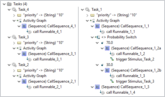
As already mentioned above, the software model of Modeling Example 2 consists exactly of four tasks, named 'Task_1' to 'Task_4'. 'Task_2' to'Task_4' call a definitive number of Runnables in a sequential order. 'Task_1' instead contains a call graph that models two different possible execution sequences. In 70% of the cases the sequence 'Runnable_1_1', 'Runnable_1_2', 'Task_2', 'Runnable_1_4' is called, while in the remaining 30% the sequence 'Runnable_1_1', 'Runnable_1_3', 'Task_3', 'Runnable_1_4' is called. As it can be seen, the call graph of 'Task_1' contains also interprocess activations, which activate other tasks.
A comprehension of the modeled properties can be found in the following table:
| Task |
Preemption |
MTA* |
Deadline |
Calls |
|
Task_1
|
Preemptive |
3 |
25 ms |
1.1) Runnable_1_1 |
| 1.2) Runnable_1_2 |
| 1.3) Task_2 |
| 1.4) Runnable_1_4 |
| 2.1) Runnable_1_1 |
| 2.2) Runnable_1_3 |
| 2.3) Task_3 |
| 2.4) Runnable_1_4 |
|
Task_2
|
Preemptive |
3 |
25 ms |
1) Runnable_2_1 |
|
Task_3
|
Preemptive |
3 |
25 ms |
1) Runnable_3_1 |
|
Task_4
|
Preemptive |
3 |
25 ms |
1) Runnable_4_1 |
*MTA = Multiple Task Activation Limit
Runnables
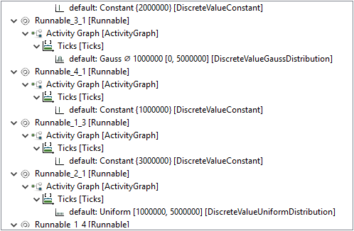
In addition to the task, the software model also contains a definition of Runnables.
For Modeling Example 2, seven individual Runnables are defined.
The only function of those in this example is to consume processing resources.
Therefore, for each Runnable a number of instruction cycles is stated.
The number of instruction cycles is thereby either constant or defined by a statistical distribution.
A comprehension of the modeled properties can be found in the following table:
| Runnable |
Type |
Instructions |
|
Runnable_1_1
|
Constant |
1000000 |
|
Runnable_1_2
|
Constant |
2000000 |
|
Runnable_1_3
|
Constant |
3000000 |
|
Runnable_1_4
|
Constant |
4000000 |
|
Runnable_2_1
|
Uniform Distribution |
1000000 |
| 5000000 |
|
Runnable_3_1
|
Gauss Distribution |
mean: 1000000 |
| sd: 50000 |
| upper: 5000000 |
|
Runnable_4_1
|
Constant |
4000000 |
Stimulation Model
The stimulation model defines the activations of tasks.
'Task_1' is activated periodically by 'Stimulus_Task_1'
'Stimulus_Task_2' and 'Stimulus_Task_3' represent the inter-process activations for the corresponding tasks.
'Task_4' finally is activated sporadically following a Gauss distribution.
A comprehension of the modeled properties can be found in the following table:
| Stimulus |
Type |
Parameters |
|
Stimulus_Task_1
|
Periodic |
offset: 0 ms |
| recurrence: 25 ms |
|
Stimulus_Task_2
|
Inter-Process |
|
|
Stimulus_Task_3
|
Inter-Process |
|
|
Stimulus_Task_4
|
Sporadic (Gauss) |
mean: 30 ms |
| sd: 5 ms |
| upper: 100 ms |
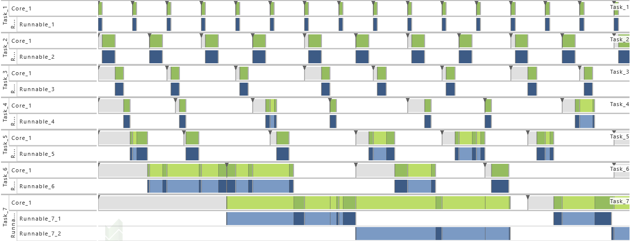
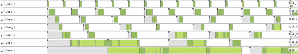
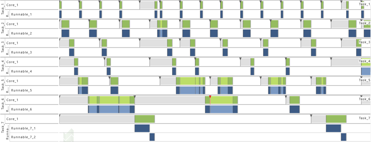
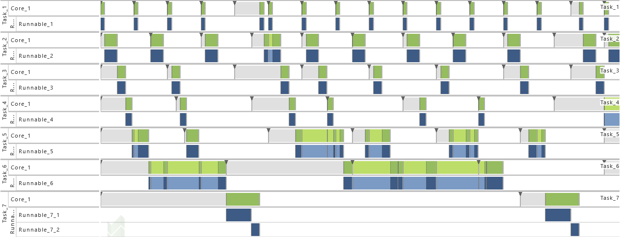
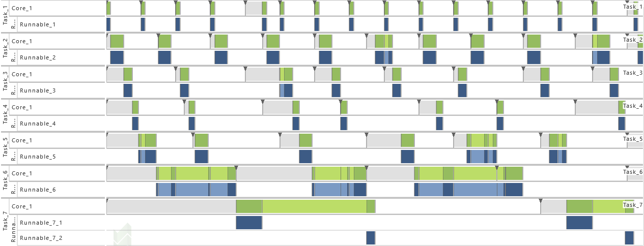
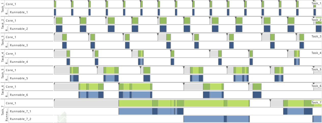
2.3.3 Modeling Example "Purely Periodic without Communication"
This system architecture pattern consists of a task set, where each task is activated periodically and no data accesses are performed. The execution time for each task is determined by the called runnable entities as specified in the table below. All tasks contain just one runnable except of T7, which calls at first R7,1 and after that R7,2.
The table below gives a detailed specification of the tasks and their parameters. The tasks are scheduled according fixed-priority, preemptive scheduling and if not indicated otherwise, all events are active in order to get a detailed insight into the system's behavior.
| Task |
Priority |
Preemption |
Multiple Task Activation Limit |
Activation |
Execution Time |
| T1 |
7 |
FULL |
1 |
Periodic |
R1 |
Uniform |
| Offset = 0 |
Min = 9.95 |
| Recurrence = 80 |
Max = 10 |
| T2 |
6 |
FULL |
1 |
Periodic |
R2 |
Uniform |
| Offset = 0 |
Min = 29.95 |
| Recurrence = 120 |
Max = 30 |
| T3 |
5 |
FULL |
1 |
Periodic |
R3 |
Uniform |
| Offset = 0 |
Min = 19.95 |
| Recurrence = 160 |
Max = 20 |
| T4 |
4 |
FULL |
1 |
Periodic |
R4 |
Uniform |
| Offset = 0 |
Min = 14.95 |
| Recurrence = 180 |
Max = 15 |
| T5 |
3 |
FULL |
1 |
Periodic |
R5 |
Uniform |
| Offset = 0 |
Min = 29.95 |
| Recurrence = 200 |
Max = 30 |
| T6 |
2 |
FULL |
1 |
Periodic |
R6 |
Uniform |
| Offset = 0 |
Min = 39.95 |
| Recurrence = 300 |
Max = 40 |
| T7 |
1 |
FULL |
1 |
|
R7,1 |
Uniform |
| Min = 59.95 |
| Periodic |
Max = 60 |
| Offset = 0 |
R7,2 |
Uniform |
| Recurrence = 1000 |
Min = 19.95 |
|
Max = 20 |
In order to show the impact of changes to the model, the following consecutive variations are made to the model:
-
1) Initial Task Set
- For this variation, the Tasks T4, T5, T6, and T7 of the table above are active.
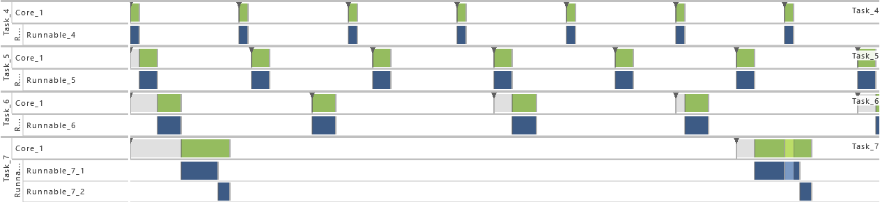
-
2) Increase of Task Set Size I
- For this variation, the Tasks T3, T4, T5, T6, and T7 are active. That way the utilization of the system is increased.
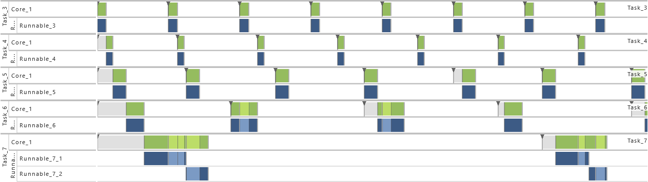
-
3) Increase of Task Set Size II
- For this variation, the Tasks T1, T3, T4, T5, T6, and T7 are active. That way the utilization of the system is increased.
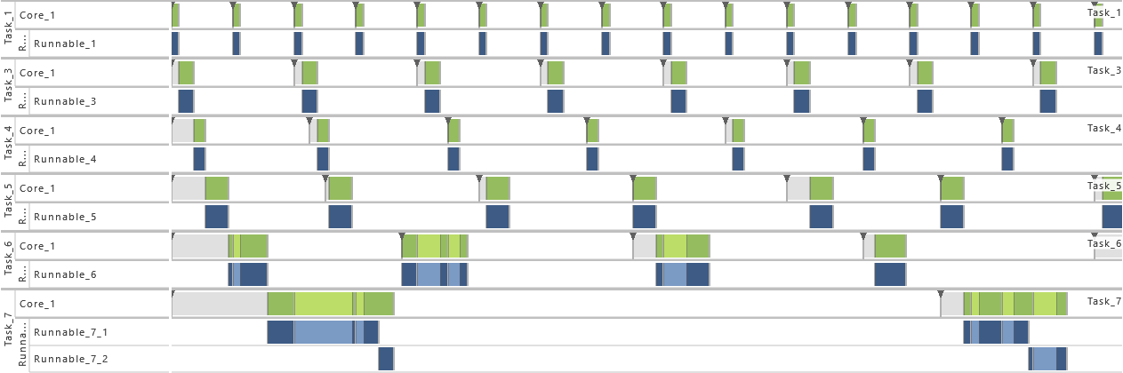
-
4) Increase of Task Set Size III
- As from this variation on, all tasks (T1 - T7) are active. That way the utilization of the system is increased.
-
5) Accuracy in Logging
- For this variation, just task events are active. That way, only a limited insight into the system's runtime behavior is available.
-
6) Schedule
- As from this variation on, T7 is set to non-preemptive. That way, the timing behavior is changed, which results in extinct activations (see red mark in the figure below).
-
7) Activation
- As from this variation on, the maximum number of queued activation requests for all tasks is set to 2. That way, the problem with extinct activations resulting from the previous variation is solved.
-
8) Schedule Point
- For this variation, a schedule point is added to T7 between the calls of R7,1 and R7,2. That way, the timing behavior is changed in particular.
-
9) Scheduling Algorithm
- For this variation, the scheduling algorithm is set to Earliest Deadline First. That way, the timing behavior is changed completely.
2.3.4 Modeling Example "Client-Server without Reply"
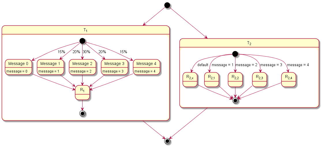
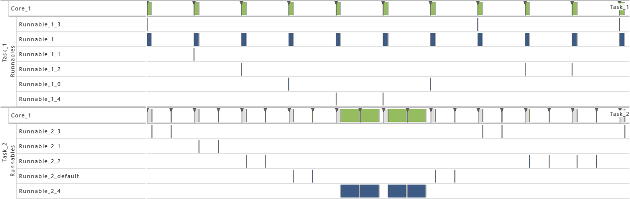
This system architecture pattern extends the modeling example "Purely Periodic without Communication" by adding an one-way communication between tasks. It consists of two tasks T1, and T2. Task T1 sends a message to Task T2 before runnable R1 is called. In 20% of the cases Message 1, in 30% of the cases Message 2, in 20% of the cases Message 3, in 15% of the cases Message 4, and in 15% of the cases any other message than the previously mentioned ones is sent. Task T2 reacts on the contents of the message by calling different runnables. In case of Message 1 runnable R2,1, in case of Message 2 runnable R2,2, in case of Message 3 runnable R2,3, in case of Message 4 runnable R2,4, and in case of any other message than the previous mentioned ones runnable R2,x is called as default.
The table below gives a detailed specification of the tasks and their parameters. The tasks are scheduled according fixed-priority, preemptive scheduling and if not indicated otherwise, all events are active in order to get a detailed insight into the system's behavior.
| Task |
Priority |
Preemption |
Multiple Task Activation Limit |
Activation |
Execution Time |
| T1 |
2 |
FULL |
1 |
Periodic |
R1 |
Uniform |
| Offset = 0 |
Min = 9.9 * 106 |
| Recurrence = 100 * 106 |
Max = 10 * 106 |
| T2 |
1 |
FULL |
1 |
|
R2,x |
Uniform |
| Min = 99 |
| Max = 100 |
| R2,1 |
Uniform |
| Min = 990 |
| Max = 1 * 103 |
| Periodic |
R2,2 |
Uniform |
| Offset = 15 * 106 |
Min = 49.5 * 103 |
| Recurrence = 60 * 106 |
Max = 50 * 103 |
|
R2,3 |
Uniform |
| Min = 990 * 103 |
| Max = 1 * 106 |
| R2,4 |
Uniform |
| Min = 39.6 * 106 |
| Max = 40 * 106 |
In order to show the impact of changes to the model, the following consecutive variations are made to the model:
-
1) Initial Task Set
- As defined by the table above.
-
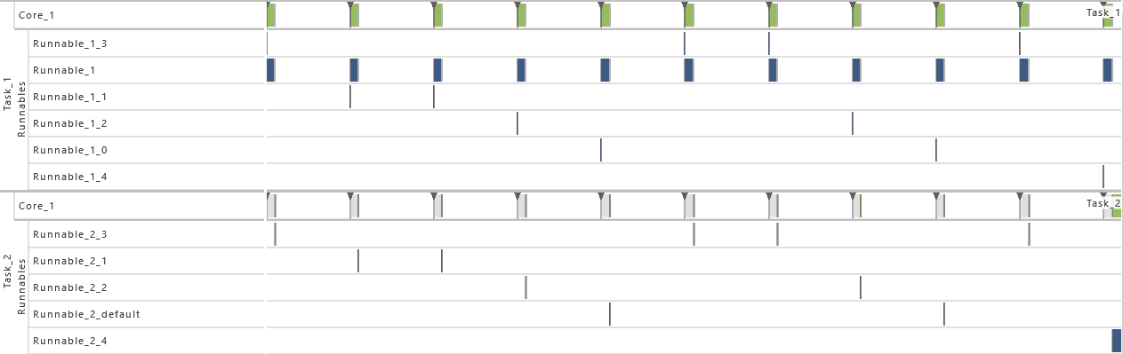
2) Exclusive Area
- For this variation, all data accesses are protected by an exclusive area. Therefore, the data accesses in T1 as well as all runnables in T2 (R2,x, R2,1, R2,2, R2,3, and R2,4) are protected during their complete time of execution via a mutex and priority ceiling protocol. That way, blocking situations appear.
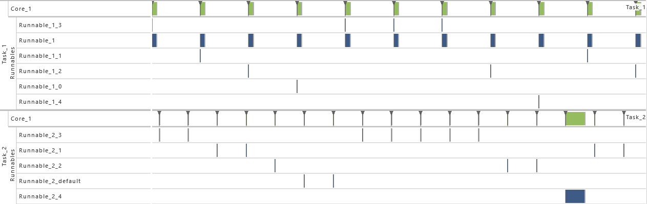
-
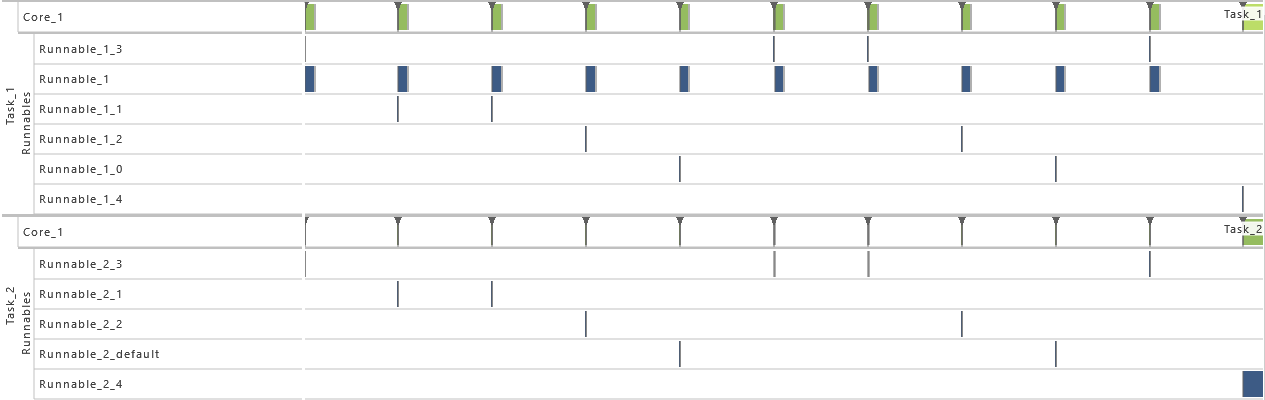
3) Inter-process Activation
- As from this variation on, task T2 gets activated by an inter-process activation from task T1 instead of being activated periodically. The interprocess activation is performed right after the message
message is written in T2 and consequently before the runnable R1 is called. That way, a direct connection between T1 and T2 is established.
-
4) Priority Ordering
- As from this variation on, the priority relation between task T1 and T2 is reversed. As a consequence, the priority of task T1 is set to 1 and the priority of task T2 is set to 2. That way, a switch from asynchronous to synchronous communication is considered.
-
5) Event Frequency Increase
- As from this variation on, the periodicity of T1 is shortened. For this, the value for the period of task T1 is cut in half to 50 * 106 time units. That way, the utilization of the system is increased.
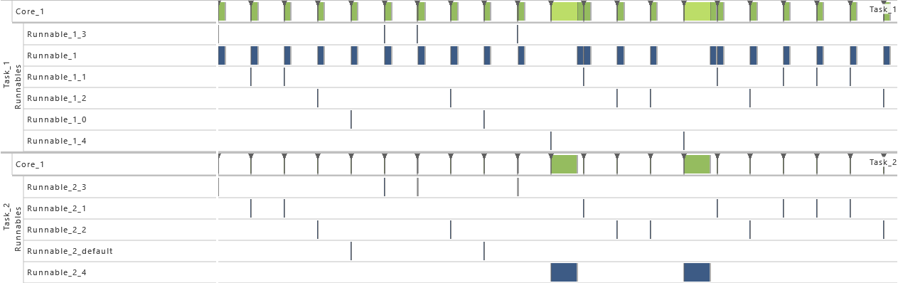
-
6) Execution Time Fluctuation
- As from this variation on, the execution time distribution is widened for both tasks. Therefore, the maximum of every uniform distribution is increased by 1 percent so that they vary now by 2 percent. That way, the utilization of the system is increased, which results in extinct activations.

-
7) Activation
- As from this variation on, the maximum number of queued activation requests for both tasks is set to 2. That way, the problem with extinct activations resulting from the previous variation is solved.
-
8) Accuracy in Logging of Data State I
- For this variation, the data accesses in task T1 and task T2 are omitted. Instead, the runnable entities R2,x, R2,1, R2,2, R2,3, and R2,4, each representing the receipt of a specific message, are executed equally random, meaning each with a probability of 20%. That way, only a limited insight into the system's runtime behavior is available.
-
9) Accuracy in Logging of Data State II
- For this variation, just task events are active. That way, only a limited insight into the system's runtime behavior is available.

2.3.5 Modeling Example "State Machine"
In this system architecture pattern the modeling example "Client Server without Reply" is extended in such a way that now the task that receives messages (T2) not only varies its dynamic behavior and consequently also its execution time according the transmitted content but also depending on its internal state, meaning the prior transmitted contents. To achieve, this task T1 sends a message to task T2 with either 0 or 1 before runnable R1 is called. The value 0 is used in 75 % of the cases and 1 in the other cases as content of the message. Starting in state 0, T2 decreases or increases the state its currently in depending on the content of the message, 0 or 1 respectively. The runnable R
2,1, R
2,2, and R
2,3 represent then the three different states that the system can be in.
The table below gives a detailed specification of the tasks and their parameters. The tasks are scheduled according fixed-priority, preemptive scheduling and if not indicated otherwise, all events are active in order to get a detailed insight into the system's behavior.
| Task |
Priority |
Preemption |
Multiple Task Activation Limit |
Activation |
Execution Time |
| T1 |
2 |
FULL |
1 |
Periodic |
R1 |
Uniform |
| Offset = 0 |
Min = 9.9 * 106 |
| Recurrence = 100 * 106 |
Max = 10 * 106 |
| T2 |
1 |
FULL |
1 |
|
R
2,1
|
Uniform |
| Min = 99 |
| Max = 100 |
| Periodic |
R
2,2
|
Uniform |
| Offset = 15 * 106 |
Min = 99 * 103 |
| Recurrence = 60 * 106 |
Max = 100 * 103 |
|
R2,3 |
Uniform |
| Min = 49.5 * 106 |
| Max = 50 * 106 |
In order to show the impact of changes to the model, the following consecutive variations are made to the model:
-
1) Initial Task Set
- As defined by the table above.
-
2) Exclusive Area
- For this variation, all data accesses are protected by an exclusive area. Therefore, the data accesses in T1 as well as all runnables in T2 (R2,1, R2,2, and R2,3) are protected during their complete time of execution via a mutex and priority ceiling protocol. That way, blocking situations appear.
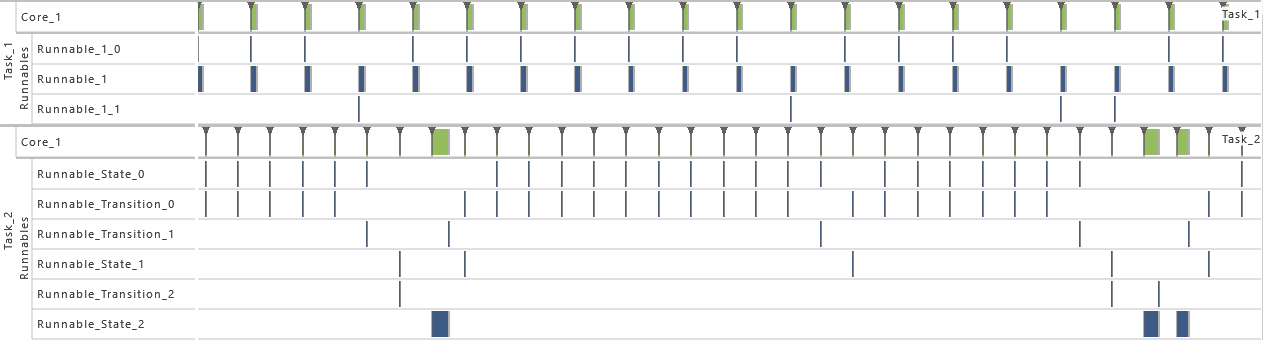
-
3) Priority Ordering
- As from this variation on, the priority relation between task T1 and T2 is reversed. As a consequence, the priority of task T1 is set to 1 and the priority of task T2 is set to 2. That way, the timing behavior is changed fully.
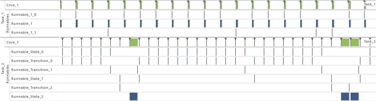
-
4) Inter-process Activation
- As from this variation on, task T2 gets activated by an inter-process activation from task T1 instead of being activated periodically. The interprocess activation is performed right after the message
message is written in T1 and consequently before the runnable R1 is called. That way, a direct connection between T1 and T2 is established.
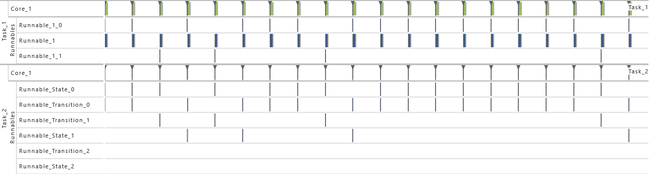
-
5) Event Frequency Increase
- As from this variation on, the periodicity of T1 is shortened. For this, the value for the period of task T1 is halved to 50 * 106. That way, the utilization of the system is increased, which results in extinct activations.
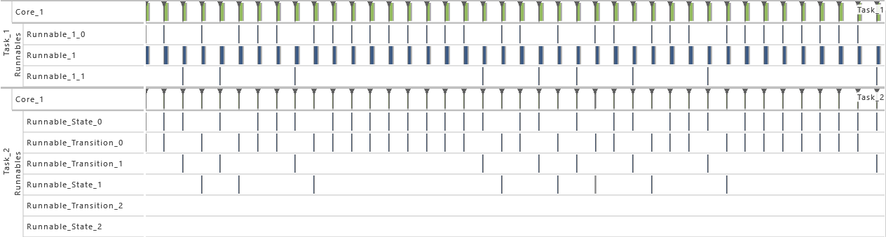
-
6) Activation
- As from this variation on, the maximum number of queued activation requests for both tasks is set to 2. That way, the problem with extinct activations resulting from the previous variation is solved.
-
7) Execution Time Fluctuation
- As from this variation on, the execution time distribution is widened for both tasks. Therefore, the maximum of the uniform distribution is increased by 1 percent so that the uniform distribution varies now by 2 percent. That way, the utilization of the system is further increased.
-
8) Accuracy in Logging of Data State I
- For this variation, the data write accesses in task T1 and task T2 are omitted. Instead, the runnables R2,1, R2,2, and R2,3, each representing the execution of a specific state, are executed with a probability of 60 %, 30 %, and 10 % respectively. That way, only a limited insight into the system's runtime behavior is available.
-
9) Accuracy in Logging of Data State II
- For this variation, just task events are active. That way, only a limited insight into the system's runtime behavior is available.

2.3.6 Modeling Example "Feedback Loop"
The task set of the modeling example "State Machine" is expanded further in this architecture pattern with the result that messages are exchanged in a loop, instead of just in one way. To achieve this, task T1 sends a message
u to task T2 before runnable R1 is called. The content of this message is 0, if the content of a previously received message
e is 0, or 1 if it was 1. Task T2 represents then a state machine with three states that increases its state, if message
u is 1 and decreases, if it is 0. In each state the messages
y and
w are set with state specific values and sent to task T3 and task T4 respectively. In case of
State 0, the messages
y and
w contain the value 0, in case of
State 1 both contain 50 and in case of
State 2 the value 100 is sent. These messages are written before runnable R2 is called. However, in 30 % of the cases task T4 is activated via an inter-process activation before this runnable call happens. Task T3 varies its dynamic behavior and consequently also its execution time according the transmitted content of message
y. Task T4 finally prepares again the input for task T1. If the content received in message
w is 0, then in 30% of the cases the content of message
e is 0, otherwise 1. In the case that message
w is 50, message
e is set to 0 with a probability of 50% and to 1 accordingly. Finally, message
e is set to 0 in 70% of the cases and to 1 in 30% of the cases, if message
w is 100. In addition to this feedback loop, other system architecture patterns are added to be executed concurrently in order to increase the complexity. The tasks T5 and T6 represent a client-server without reply and are equal to the tasks T1 and T2 respectively as described in the modeling example "Client-Server without Reply". T7 is a periodically activated task without any communication and identical to task T7 of modeling example "Purely Periodic without Communication".
The table below gives a detailed specification of the tasks and their parameters. The tasks are scheduled according fixed-priority, preemptive scheduling and if not indicated otherwise, all events are active in order to get a detailed insight into the system's behavior.
| Task |
Priority |
Preemption |
Multiple Task Activation Limit |
Activation |
Execution Time |
| T1 |
3 |
FULL |
1 |
Periodic |
R1 |
Uniform |
| Offset = 0 |
Min = 9.9 * 106 |
| Recurrence = 600 * 106 |
Max = 10 * 106 |
| T2 |
2 |
FULL |
1 |
Periodic |
R2 |
Uniform |
| Offset = 20 * 106 |
Min = 99 * 104 |
| Recurrence = 300 * 106 |
Max = 100 * 104 |
| T3 |
3 |
FULL |
1 |
|
R3,0 |
Uniform |
| Min = 99 * 104 |
| Max = 100 * 104 |
| Periodic |
R3,1 |
Uniform |
| Offset = 50 * 106 |
Min = 99 * 105 |
| Recurrence = 500 * 106 |
Max = 100 * 105 |
|
R3,2 |
Uniform |
| Min = 99 * 106 |
| Max = 100 * 106 |
| T4 |
1 |
FULL |
1 |
|
R4 |
Uniform |
| Inter-process Activation |
Min = 99 * 105 |
|
Max = 100 * 105 |
| T5 |
5 |
FULL |
1 |
Periodic |
R5 |
Uniform |
| Offset = 0 |
Min = 99 * 105 |
| Recurrence = 100 * 106 |
Max = 100 * 105 |
| T6 |
4 |
FULL |
1 |
|
R6,x |
Uniform |
| Min = 99 |
| Max = 100 |
| R6,1 |
Uniform |
| Min = 990 |
| Max = 1 * 103 |
| Periodic |
R6,2 |
Uniform |
| Offset = 15 * 106 |
Min = 49.5 * 103 |
| Recurrence = 60 * 106 |
Max = 50 * 103 |
|
R6,3 |
Uniform |
| Min = 990 * 103 |
| Max = 1 * 106 |
| R6,4 |
Uniform |
| Min = 49.5 * 106 |
| Max = 50 * 106 |
| T7 |
0 |
FULL |
1 |
|
R7,1 |
Uniform |
| Min = 59.4 * 106 |
| Periodic |
Max = 60 * 106 |
| Offset = 0 |
R7,2 |
Uniform |
| Recurrence = 1000 |
Min = 19.8 * 106 |
|
Max = 20 * 106 |
In order to show the impact of changes to the model, the following consecutive variations are made to the model:
-
1) Initial Task Set
- For this variation, the tasks T1, T2, T3, and T4 of the table above are active.
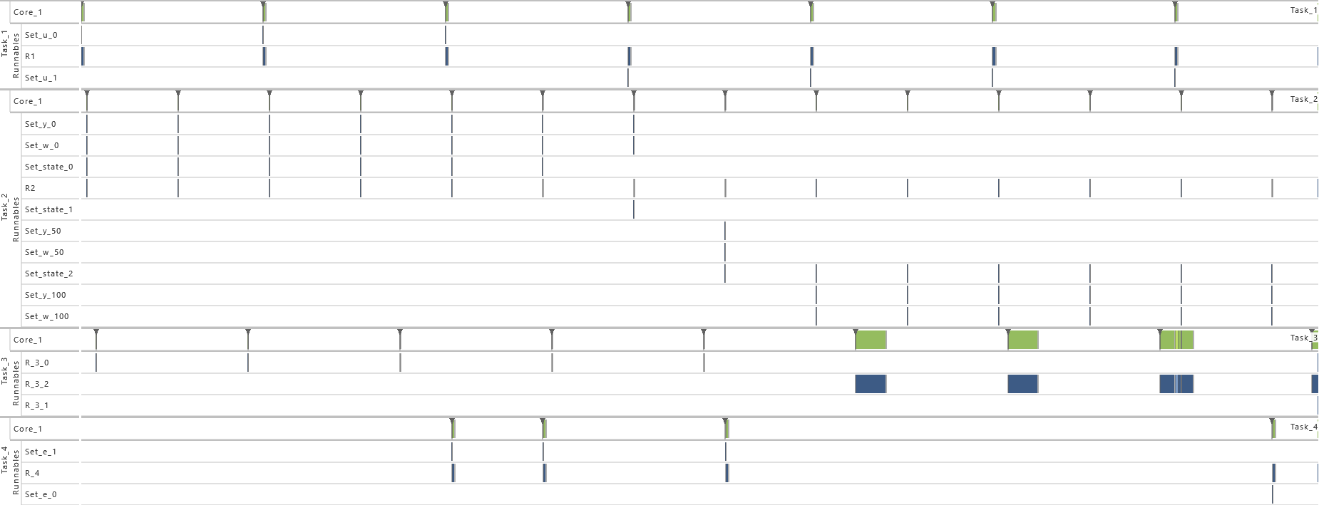
-
2) Increase of Task Set Size I
- For this variation, the Tasks T1, T2, T3, T4, T5, and T6 are active. That way the utilization of the system is increased.
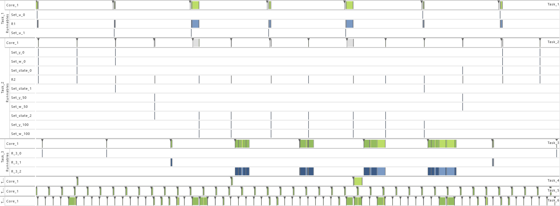
-
3) Increase of Task Set Size II
- As from this variation on, all tasks are active. That way the utilization of the system is increased.
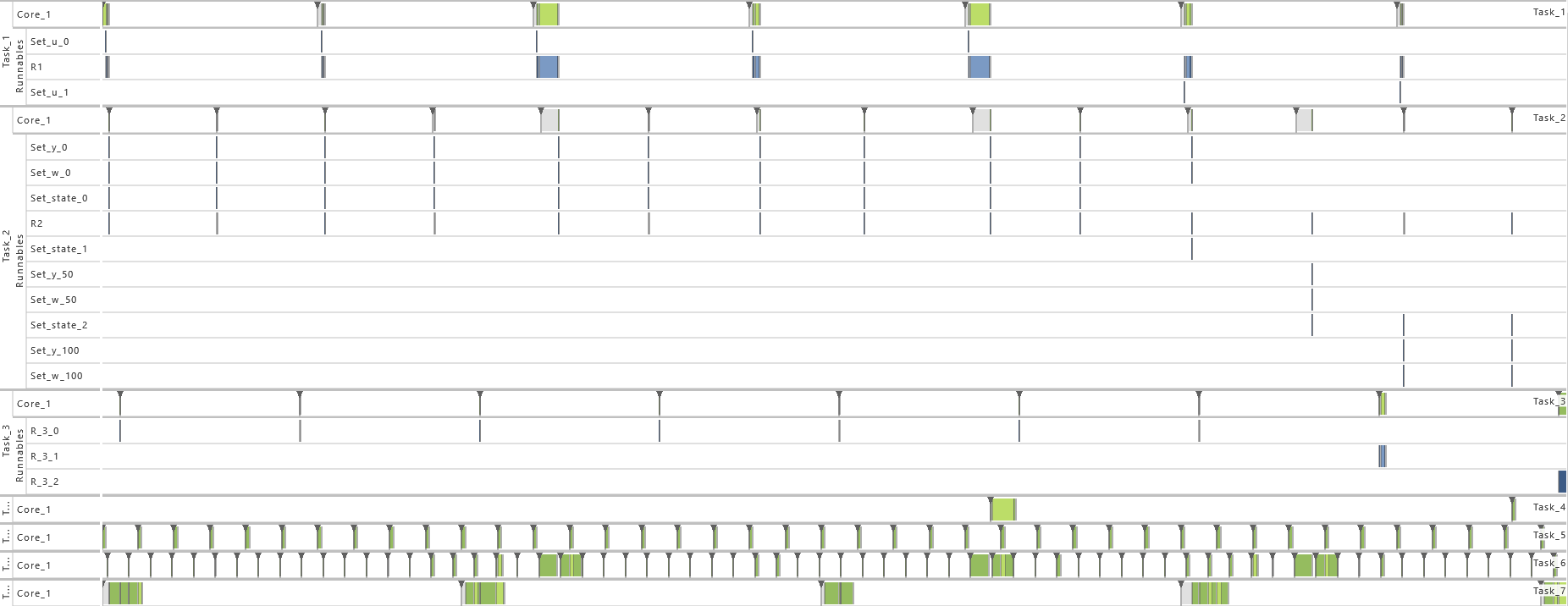
-
4) Inter-process Activation
- As from this variation on, task T2 gets activated by an inter-process activation from task T1, task T3 by an inter-process activation from task T2, and task T6 by an inter-process activation from task T5 instead of being activated periodically. The inter-process activation in task T1 is performed right after the message
u is written in T2 and consequently before the runnable R1 is called, in task T2 respectively right before task T4 is activated, and in task T5 task T6 is called right before runnable R5. That way, a direct connection between these tasks is established.
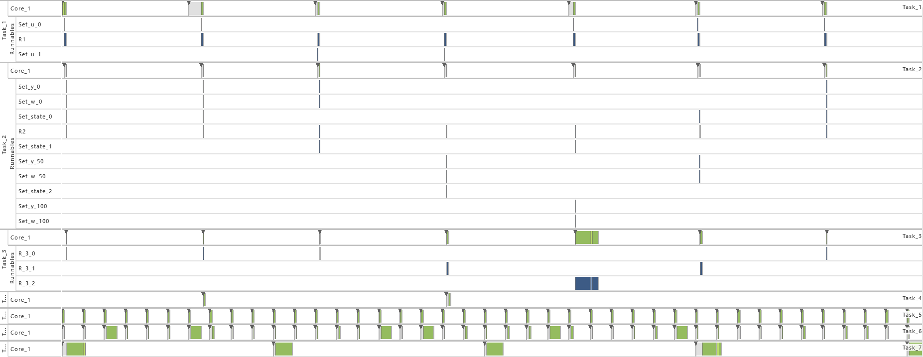
-
5) Event Frequency Increase
- As from this variation on, the periodicity of the tasks T1, T5, and T7 are shortened. For task T1, the value for the period is set to 450 * 106, the task T5 to 60 * 106, and for task T7 to 575 * 106. That way, the information density is increased.
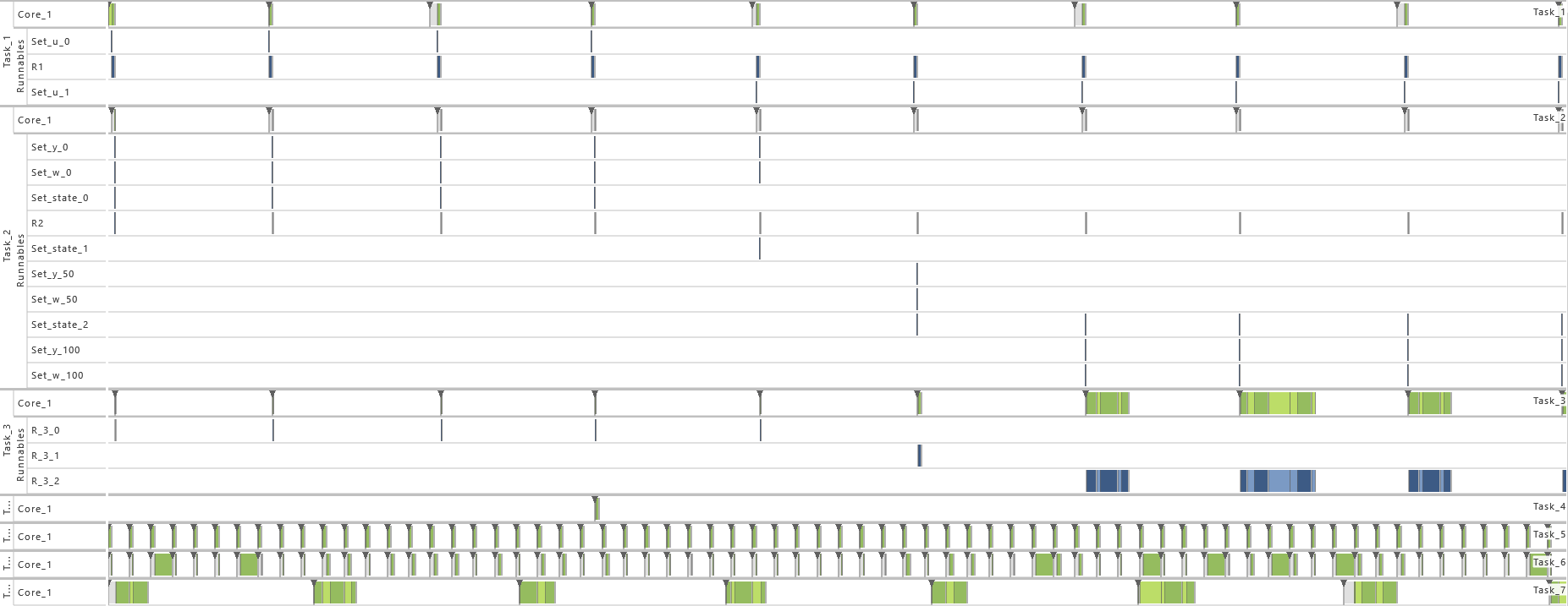
-
6) Execution Time Fluctuation
- As from this variation on, the execution time distribution is widened for both tasks. Therefore, the maximum of the uniform distribution is increased by 1 percent so that the uniform distribution varies now by 2 percent. That way, the utilization of the system is increased, which results in extinct activations.
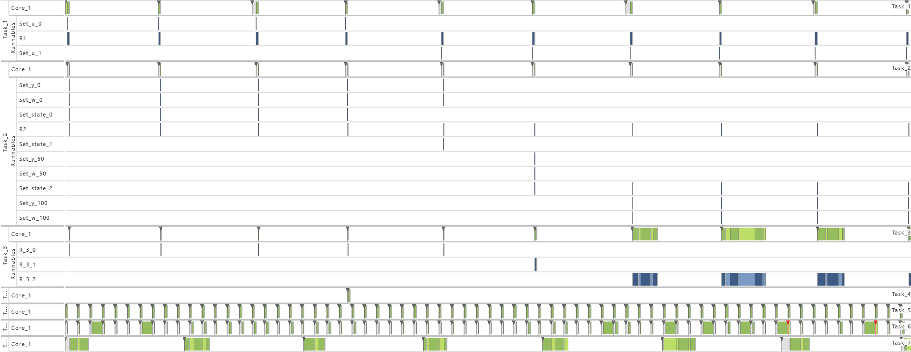
-
7) Activation
- As from this variation on, the maximum number of queued activation requests for both tasks is set to 2. That way, the problem with extinct activations resulting from the previous variation is solved.
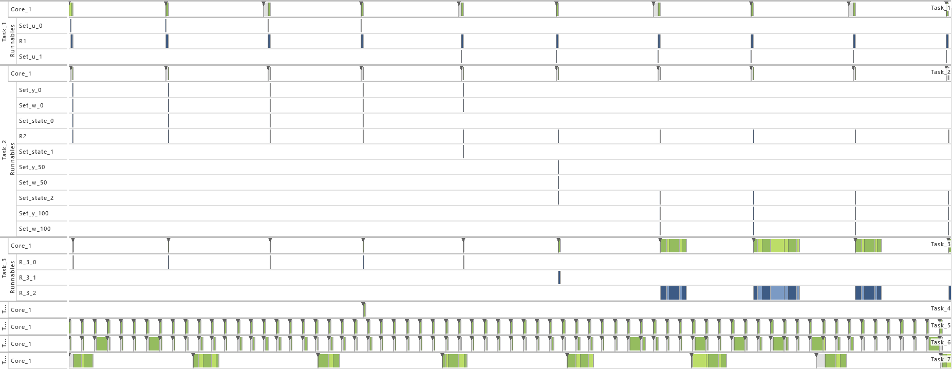
-
8) Accuracy in Logging of Data State I
- For this variation, the data accesses in all tasks are omitted. Instead, the runnable entities R3,0, R3,1, and R3,2, are executed with a probability of 50 %, 30 %, and 20 % respectively, and the runnable entities R6,x, R6,1, R6,2, R6,3, and R6,4 are executed with a probability of 15 %, 20 %, 30 %, 20 %, and 15 % respectively. That way, only a limited insight into the system's runtime behavior is available.
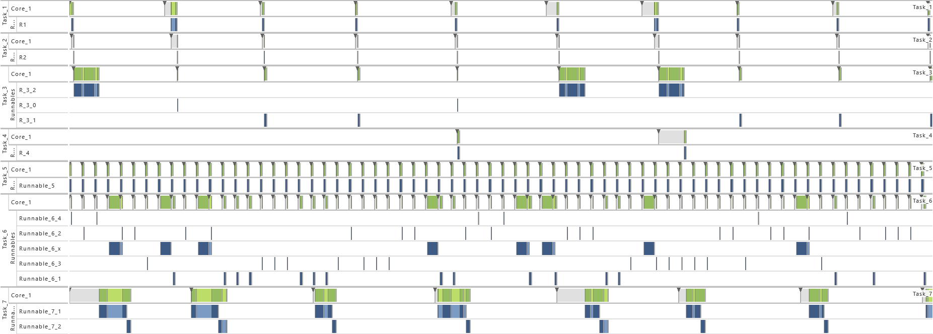
-
9) Accuracy in Logging of Data State II
- For this variation, just task events are active. That way, only a limited insight into the system's runtime behavior is available.
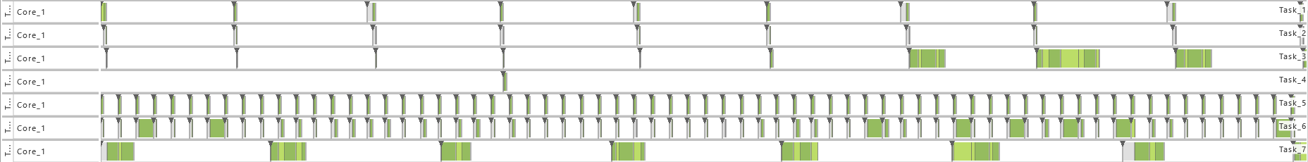
2.3.7 Modeling Example "State Machine Feedback Loop"
The task set of the modeling example "State Machine" is expanded further in this architecture pattern by combining the ideas behind the modeling example "State Machine" and "Feedback Loop". This means that messages are exchanged in a loop and each sender/receiver is also a state machine. To achieve this, task T1 has two different internal states 0 and 1, and task T2 manages three consecutive states 0, 1, and 2. The state task T1 is currently in is sent via a message to task T2 before runnable R1 is called. If the content of the message sent from task T1 is 1, task T2 increases its internal state, e.g. from state 0 to 1, and if it is 0, task T2 decreases its internal state accordingly. Then, depending on the state task T2 is currently in, the according runnable (R2,0 for state 0, etc.) is executed. If the maximum or minimum state of task T2 is reached but the received message from task T1 tells task T2 to further increase or respectively decrease its internal state, task T2 sends a message to task T1. This message then causes task T1 to toggle its internal state which consequently results in a switch from increasing to decreasing or vice versa. In addition to this state machine feedback loop, other system architecture patterns are added to be executed concurrently in order to increase the complexity. The tasks T3 and T4 represent a client-server without reply and are equal to the tasks T1 and T2 respectively as described above in the modeling example "Client-Server without Reply". T5 is a periodically activated task without any communication and identical to task T7 in the modeling example "Purely Periodic without Communication".
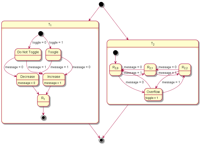
The table below gives a detailed specification of the tasks and their parameters. The tasks are scheduled according fixed-priority, preemptive scheduling and if not indicated otherwise, all events are active in order to get a detailed insight into the system's behavior.
| Task |
Priority |
Preemption |
Multiple Task Activation Limit |
Activation |
Execution Time |
| T1 |
2 |
FULL |
1 |
Periodic |
R1 |
Uniform |
| Offset = 0 |
Min = 9.9 * 106 |
| Recurrence = 300 * 106 |
Max = 10 * 106 |
| T2 |
1 |
FULL |
1 |
|
R2,0 |
Uniform |
| Min = 99 |
| Max = 100 |
| Periodic |
R2,1 |
Uniform |
| Offset = 15 * 106 |
Min = 99 * 103 |
| Recurrence = 250 * 106 |
Max = 100 * 103 |
|
R2,2 |
Uniform |
| Min = 49.5 * 106 |
| Max = 50 * 106 |
| T3 |
4 |
FULL |
1 |
Periodic |
R3 |
Uniform |
| Offset = 0 |
Min = 99 * 105 |
| Recurrence = 100 * 106 |
Max = 100 * 105 |
| T4 |
3 |
FULL |
1 |
|
R4,x |
Uniform |
| Min = 99 |
| Max = 100 |
| R4,1 |
Uniform |
| Min = 990 |
| Max = 1 * 103 |
| Periodic |
R4,2 |
Uniform |
| Offset = 15 * 106 |
Min = 49.5 * 103 |
| Recurrence = 60 * 106 |
Max = 50 * 103 |
|
R4,3 |
Uniform |
| Min = 990 * 103 |
| Max = 1 * 106 |
| R4,4 |
Uniform |
| Min = 49.5 * 106 |
| Max = 50 * 106 |
| T5 |
0 |
FULL |
1 |
|
R5,1 |
Uniform |
| Min = 59.4 * 106 |
| Periodic |
Max = 60 * 106 |
| Offset = 0 |
R5,2 |
Uniform |
| Recurrence = 1000 |
Min = 19.8 * 106 |
|
Max = 20 * 106 |
In order to show the impact of changes to the model, the following consecutive variations are made to the model:
-
1) Initial Task Set
- For this variation, the tasks T1, and T2 of the table above are active.
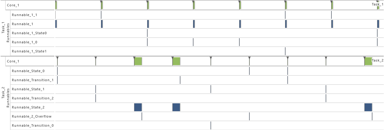
-
2) Increase of Task Set Size I
- For this variation, the tasks T1, T2, T3, and T4 are active. That way the utilization of the system is increased.
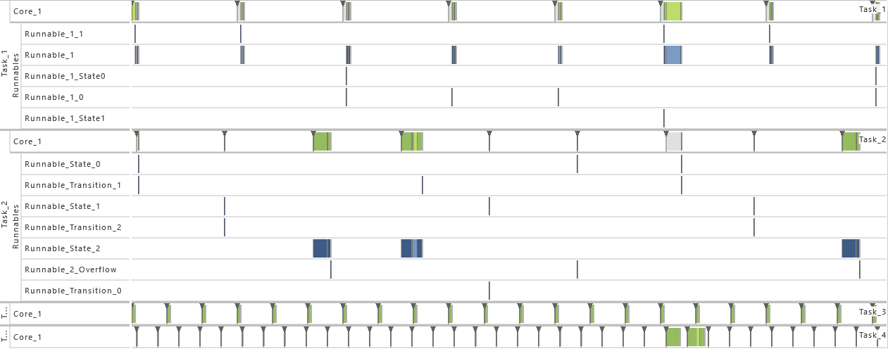
-
3) Increase of Task Set Size II
- As from this variation on, all tasks are active. That way the utilization of the system is increased.
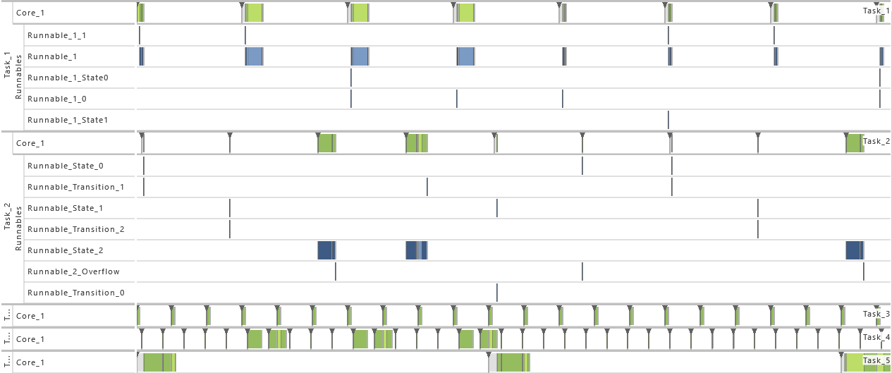
-
4) Inter-process Activation
- As from this variation on, task T2 gets activated by an inter-process activation from task T1, and task T4 by an inter-process activation from task T3 instead of being activated periodically. The inter-process activation in task T1 is performed right after the message to task T2 is written and consequently before the runnable R1 is called, and in task T3 task T4 is called right before runnable R3. That way, a direct connection between these tasks is established.
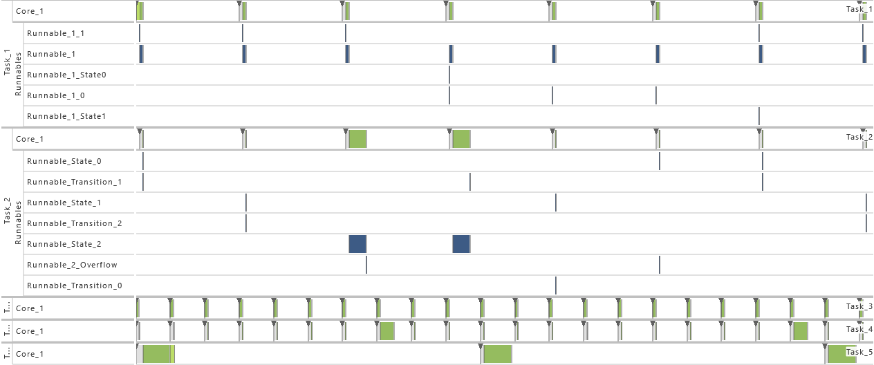
-
5) Event Frequency Increase
- As from this variation on, the periodicity of the tasks T1, T3, and T5 are shortened. For task T1, the value for the period is set to 220 * 106, the task T3 to 50 * 106, and for task T5 to 500 * 106. That way, the information density is increased.
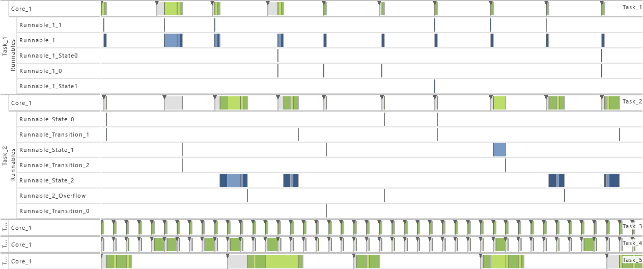
-
6) Execution Time Fluctuation
- As from this variation on, the execution time distribution is widened for both tasks. Therefore, the maximum of the uniform distribution is increased by 1 percent so that the uniform distribution varies now by 2 percent. That way, the utilization of the system is increased, which results in extinct activations.
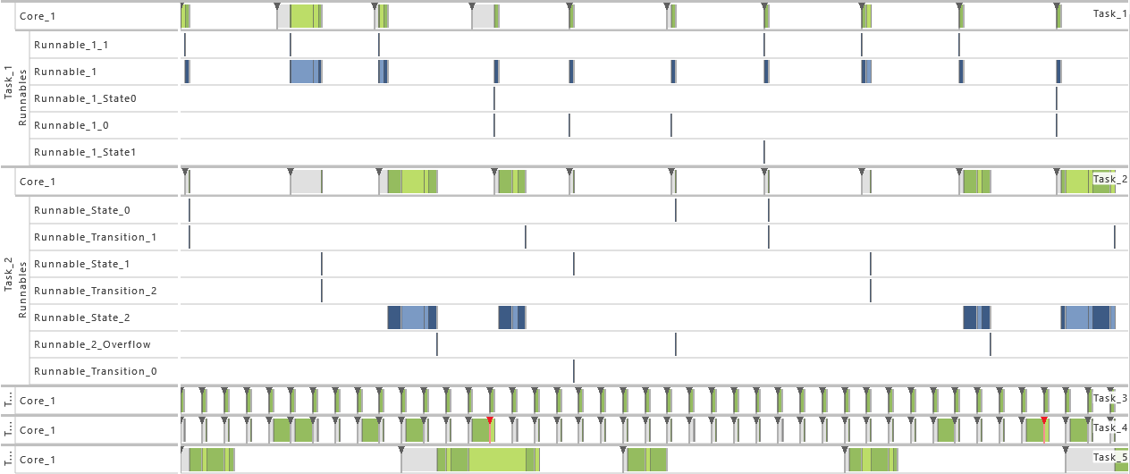
-
7) Activation
- As from this variation on, the maximum number of queued activation requests for both tasks is set to 2. That way, the problem with extinct activations resulting from the previous variation is solved.
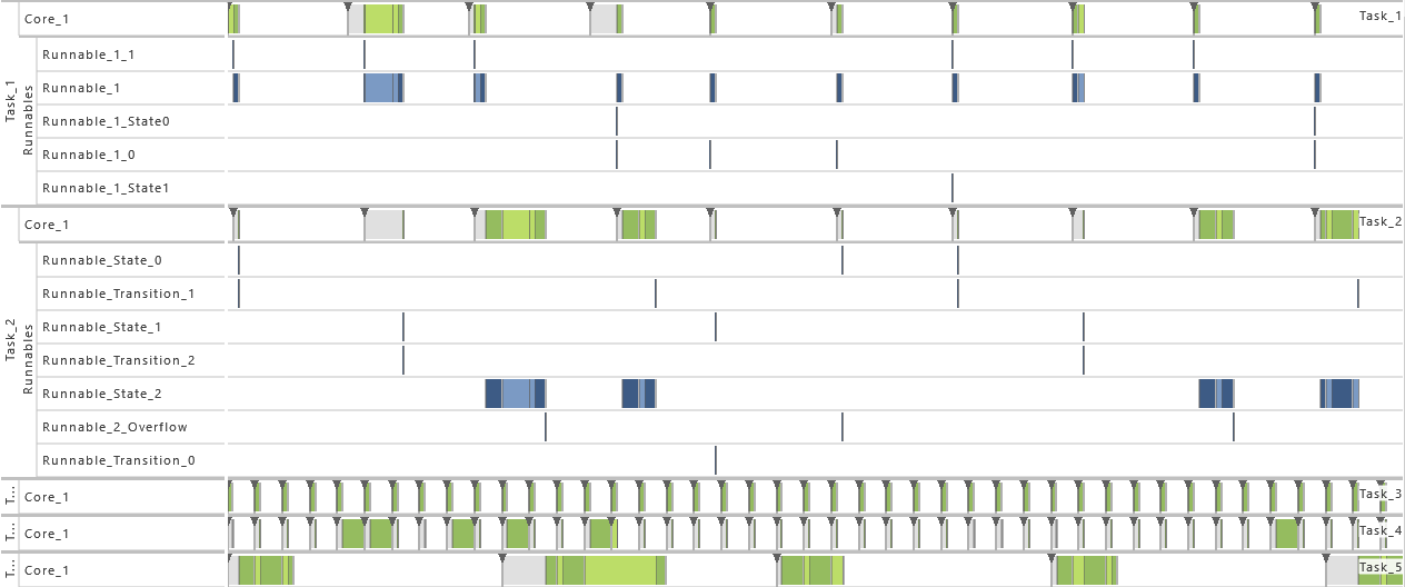
-
8) Accuracy in Logging of Data State I
- For this variation, the data accesses in all tasks are omitted. Instead, all runnablea representing a state are executed equally random, meaning the runnables R2,0, R2,1, and R2,2 are each executed with a probability of 33 %, and the runnables R4,x, R4,1, R4,2, R4,3, and R4,4 each with a probability of 20 %. That way, only a limited insight into the system's runtime behavior is available.
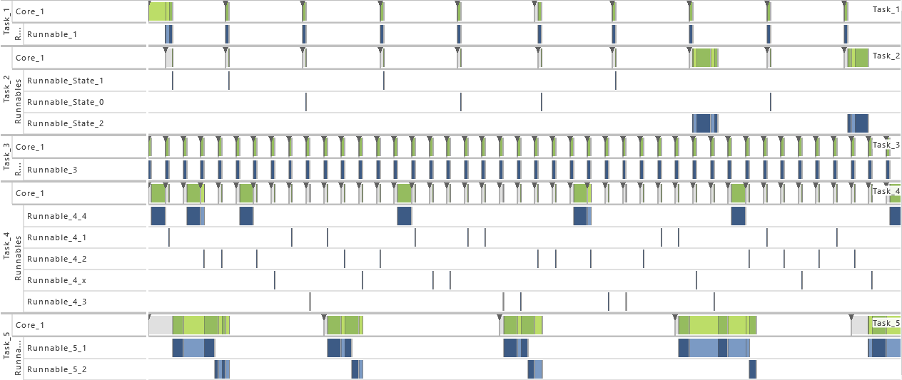
-
9) Accuracy in Logging of Data State II
- For this variation, just task events are active. That way, only a limited insight into the system's runtime behavior is available.
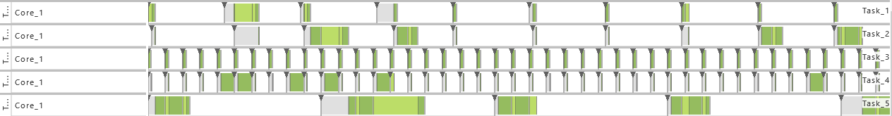
2.3.8 Democar Example
The so called Democar model presented in the AMALTHEA example files describe a simple engine management system.
Origin
The Democar example is loosely based on the publicly available information taken from
A Timing Model for Real-Time Control-Systems and its Application
on Simulation and Monitoring of AUTOSAR Systems
Author: Patrick Frey
A version of the dissertation can be downloaded from University of Ulm:
pdf.
Files
democar.amxmi
contains the complete model, consisting of a hardware model, a model of the operating system, a stimulation model and a model that describes the software system.
trace-example.atdb
is an AMALTHEA Trace Database and it contains a trace that is the result of a simulation of this example.
2.3.9 Hardware Examples
This example contains two simple hardware models:
Example 1: Simple_ECU
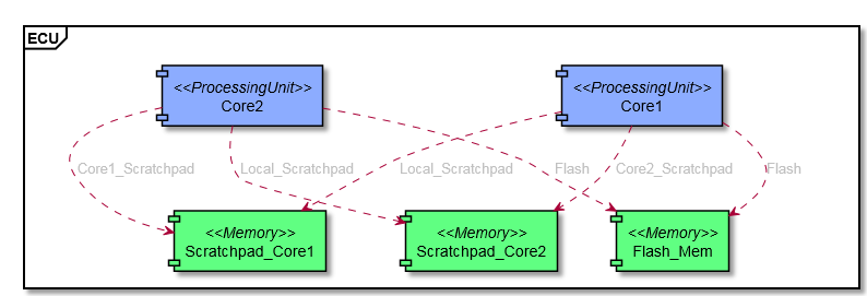
The example shows a single structure with two identical cores with such an Instruction per cycle feature. The model includes only one frequency domain and no power domain. Each core is connected to all three different memory units via a
HwAccessElement with read and write latencies. The memory components include an access latency. This means the total latency for a read and a write access are calculated in the following way:
TotalReadLatency = readLatency + accessLatency
TotalWriteLatency = writeLatency + accessLatency
This example shows a very simple hardware modeling approach where no interconnects and ports are necessary. Such a model can be used in a very early design phase where only rough estimations or a limited amount of informations about the system are available.
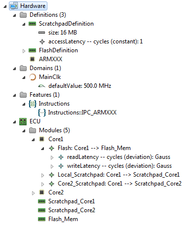
Example 2: Simple_E_E_Architecture
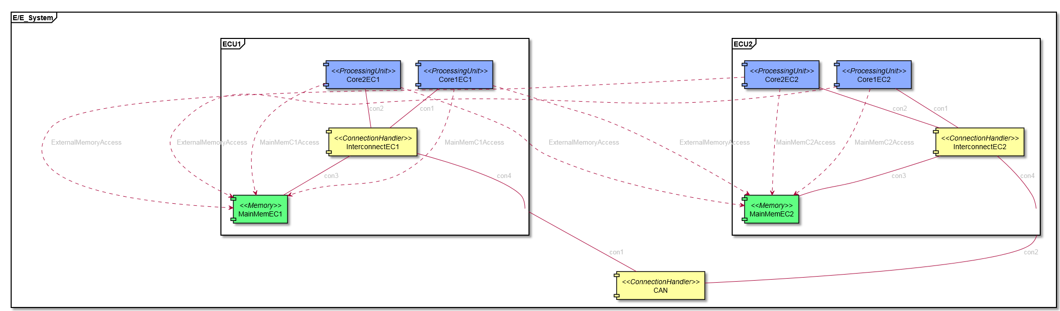
The second example shows a simple E/E-Architecture out of two identical ECUs. Each ECU contains two cores, one interconnect and a memory component. Both ECUs are connected via a CAN-Bus. In this example both possibilities for a
HwAccessElement are shown. The local memory is just connected with read and write latencies and the external memory of the other ECU is connected with the help of a
HwAccessPath. To use access paths hardware ports and connections between those ports are mandatory. The access paths itself is an ordered list of elements which are used for the connection. As an example for the access path between Core1EC1 and MainMemEC2 following access path elements are referred:
con1 -> internalCan_ECU1 -> con4 -> con9 -> CAN -> con10 -> con8 -> InterconnectEC2 -> con7.
That means the complete access paths includes:
- 3 x ConnectionHandler
- 6 x HwConnections
The latency in this case is the sum of all elements of the path plus the access latency of the memory. However latencies at connections are usually only used to account an offset for a specific component. In case a data rate is used the maximum data rate is limited by the lowest data rate in the path. In case of a
ConnectionHandler the data rate is usually shared between different accesses.
The hierarchical ports from both ECUs to connect the CAN Bus with the ECUs as block boxes are not mandatory but recommended. This concept of hierarchical ports increases the number of HwConnections but allows also the structuring of all internal modules within a HwStructure and only connect the hierarchical ports with the rest of the system.
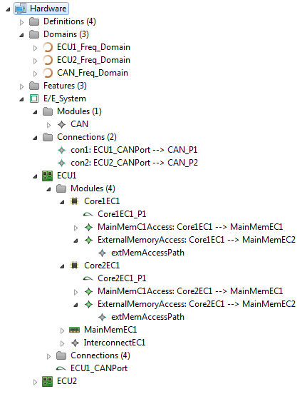
2.3.10 Scheduler Examples
The following elements are used to illustrate the structure of the example schedulers:
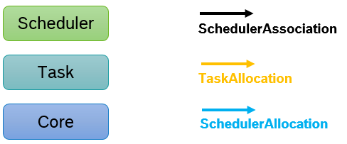
Hierarchical Scheduler
In this example the main scheduler realizes a
Priority Round Robin strategy. The main scheduler works as a global scheduler that schedules subsystems like virtual machines or hypervisor partitions. Each partition realizes an
OSEK scheduling system. In this case the main scheduler is responsible for both cores but only running on one core. Each
OSEK subsystem is responsible for exactly one core but only if the main scheduler grants the core usage. The
OSEK subsystems then decide on a FPP basis, which task can run. The coreAffinity for the tasks is not needed, since their scheduler is only responsible for one core.
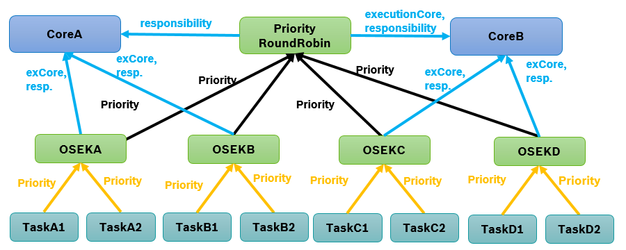
Partitioned_FPP Scheduler
In this example an FPP scheduler acts as a global scheduler. It schedules tasks on a FPP basis but with the additional constraint that its group must have budget left (has similarities to 'adaptive partitioned scheduling' of QNX). The scheduler "CBS" (Constant Bandwith Server) is only there to assign budgets to a logical task group and define no mapping or responsibility at all. Therefore, in the taskAllocation only the priority is specified. The coreAffinity of tasks in the same group can differ, even task migration is possible if a task affinity is
CoreA as well as
CoreB.

2.3.11 Numeric Modes Example
Dynamic task activations and the execution of different control paths can depend on internal system states, external events and scheduling effects resulting in different execution sequences of tasks. In APP4MC modes can be used to steer different execution paths. The designer can define modes that execute different paths within runnables, tasks, and even control dynamic activation schemes of tasks with multiple dependencies. This page explains the concepts with a simple example. For the description of the basic model elements, we refer the reader to the chapters:
Data Models -> Software Model -> Modes
Data Models -> Software Model -> Runnable Items -> Runnable Mode Switch
Data Models -> Software Model -> The Call Graph -> Mode Switch
Data Models -> Stimuli Model -> Mode Value List and Execution Condition
Example description
In this chapter, we show a small example how to use modes to steer the execution and the activation of tasks with modes. The following picture depicts the example:
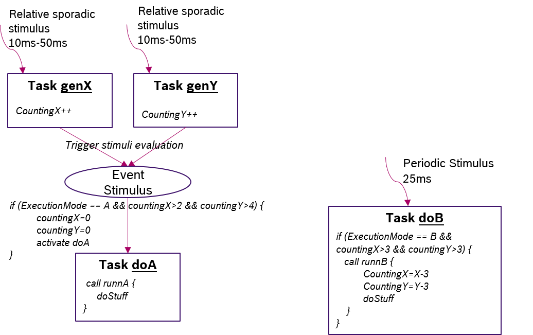
In this example, we have three modes, one _Enum__ and two
Numeric. The numeric modes are initialized with the value -1:
First, we have two data generators with Task
genX and Task
genY where each execution increases a numeric mode by 1. They are activated by a relative sporadic stimulus with an occurrence interval between 10ms and 50ms. The runnable
counterForX executes this for
genX:
On every execution, the generator tasks trigger the
CustomEvent
check to evaluate the
EventStimulus. This event stimulus checks the condition:
executionMode == ModeA && countX > 2 && countY > 4
In this example, we do not describe the change of the
executionMode to keep the model simpler. This mode could be changed e.g. from within the system or by an external ISR trigger.
If this condition is true, both counting modes are set to zero and the Task
doA is called.
Another way to steer the execution depending can be done via mode switches on task level. In
doB the mode check is done at task level as depicted in the following picture:
Only if the condition is true runnable
runB is called. Within this runnable the counting modes are decremented by 3.
The last mechanisms is also possible at runnable level by using the
runnableModeSwitch.
Beware of where to reset or change the modes. In
doB the modes are reseted directly in the beginning. If you by accident put these after the
tick element, it could result in an unintended behavior. In the generator tasks be aware of where to put the
customEventTrigger. This element activates the stimuli evaluation. If you put a tick element between the increment and the trigger, the evaluation is delayed.
2.3.12 AMALTHEA Trace Database (ATDB) Example
The ATDB provides tables and view definitions to hold trace data and represent it in comprehensive views. In this section we will show a small example BTF trace, convert it to its ATDB equivalent, and enrich it with event chains. The relevant tables and views will given for better understanding.
Source BTF Trace
The source BTF trace has two cores, three stimuli, three tasks, and four runnables.
#version 2.1.5
#timeScale ns
0,ECU_1,-1,SIM,SIM,-1,tag,ECU_INIT
0,Processor_1,-1,SIM,SIM,-1,tag,PROCESSOR_INIT
0,Core_1,-1,SIM,SIM,-1,tag,CORE_INIT
0,Core_2,-1,SIM,SIM,-1,tag,CORE_INIT
0,Core_1,0,C,Core_1,0,set_frequence,10000000
0,Core_2,0,C,Core_2,0,set_frequence,11000000
0,Stimulus_Task_1,0,STI,Stimulus_Task_1,0,trigger
0,Stimulus_Task_1,0,T,Task_1,0,activate
0,Stimulus_Task_2,0,STI,Stimulus_Task_2,0,trigger
0,Stimulus_Task_2,0,T,Task_2,0,activate
100,Core_1,0,T,Task_1,0,start
100,Task_1,0,R,Runnable_1_1,0,start
100,Core_2,0,T,Task_2,0,start
100,Task_2,0,R,Runnable_2_1,0,start
20800,Task_1,0,R,Runnable_1_1,0,terminate
20800,Task_1,0,R,Runnable_1_2,0,start
40900,Task_1,0,R,Runnable_1_2,0,terminate
40900,Core_1,0,T,Task_1,0,terminate
45000,Stimulus_Task_3,0,STI,Stimulus_Task_3,0,trigger
45000,Stimulus_Task_3,0,T,Task_3,0,activate
45100,Task_2,0,R,Runnable_2_1,0,suspend
45100,Core_2,0,T,Task_2,0,preempt
45100,Core_2,0,T,Task_3,0,start
45100,Task_3,0,R,Runnable_3_1,0,start
55800,Task_3,0,R,Runnable_3_1,0,terminate
55800,Core_2,0,T,Task_3,0,terminate
55900,Core_2,0,T,Task_2,0,resume
55900,Task_2,0,R,Runnable_2_1,0,resume
61000,Task_2,0,R,Runnable_2_1,0,terminate
61000,Core_2,0,T,Task_2,0,terminate
There is exacly one instance of each entity in the trace, so the tables in the database do not become to big for a small example. The visualized Gantt chart of the above trace is depicted in the following figure:
Equivalent ATDB Contents
The tables and/or relevant views for the above BTF trace are listed in the following: Note that if the table's header starts with a "v" it is a view for better readability.
|
MetaInformation
|
| name |
value |
| timeBase |
ns |
|
Entity
|
| id |
name |
entityTypeId |
| 1 |
SIM |
1 |
| 2 |
ECU_1 |
2 |
| 3 |
Processor_1 |
3 |
| 4 |
Core_1 |
4 |
| 5 |
Core_2 |
4 |
| 6 |
Stimulus_Task_1 |
5 |
| 7 |
Task_1 |
6 |
| 8 |
Stimulus_Task_2 |
5 |
| 9 |
Task_2 |
6 |
| 10 |
Runnable_1_1 |
7 |
| 11 |
Runnable_2_1 |
7 |
| 12 |
Runnable_1_2 |
7 |
| 13 |
Stimulus_Task_3 |
5 |
| 14 |
Task_3 |
6 |
| 15 |
Runnable_3_1 |
7 |
|
EntityInstance
|
| entityId |
sqcnr |
| 1 |
-1 |
| 2 |
-1 |
| 3 |
-1 |
| 4 |
-1 |
| 4 |
0 |
| 5 |
-1 |
| 5 |
0 |
| 6 |
0 |
| 7 |
0 |
| 8 |
0 |
| 9 |
0 |
| 10 |
0 |
| 11 |
0 |
| 12 |
0 |
| 13 |
0 |
| 14 |
0 |
| 15 |
0 |
|
EntityType
|
| id |
name |
| 1 |
SIM |
| 2 |
ECU |
| 3 |
Processor |
| 4 |
C |
| 5 |
STI |
| 6 |
T |
| 7 |
R |
|
Property
|
| id |
name |
type |
| 1 |
processors |
entityIdRef |
| 2 |
cores |
entityIdRef |
| 3 |
frequencyInHz |
long |
| 4 |
stimuli |
entityIdRef |
| 5 |
executingCore |
entityIdRef |
| 6 |
runnables |
entityIdRef |
| 7 |
ecItems |
entityIdRef |
| 8 |
ecStimulus |
eventIdRef |
| 9 |
ecResponse |
eventIdRef |
| 10 |
ecMinItemsCompleted |
long |
Note that in the entityInstance table there are actually two instances of the cores (entityIds 4 and 5). Also note, the event chain properties are already contained in the property table.
|
vTraceEvent
|
| timestamp |
sqcnr |
entityName |
entityType |
entityInstance |
sourceEntityName |
sourceEntityType |
sourceEntityInstance |
eventType |
value |
| 0 |
0 |
Stimulus_Task_1 |
STI |
0 |
Stimulus_Task_1 |
STI |
0 |
trigger |
|
| 0 |
1 |
Task_1 |
T |
0 |
Stimulus_Task_1 |
STI |
0 |
activate |
|
| 0 |
2 |
Stimulus_Task_2 |
STI |
0 |
Stimulus_Task_2 |
STI |
0 |
trigger |
|
| 0 |
3 |
Task_2 |
T |
0 |
Stimulus_Task_2 |
STI |
0 |
activate |
|
| 100 |
0 |
Task_1 |
T |
0 |
Core_1 |
C |
0 |
start |
|
| 100 |
1 |
Runnable_1_1 |
R |
0 |
Task_1 |
T |
0 |
start |
|
| 100 |
2 |
Task_2 |
T |
0 |
Core_2 |
C |
0 |
start |
|
| 100 |
3 |
Runnable_2_1 |
R |
0 |
Task_2 |
T |
0 |
start |
|
| 20800 |
0 |
Runnable_1_1 |
R |
0 |
Task_1 |
T |
0 |
terminate |
|
| 20800 |
1 |
Runnable_1_2 |
R |
0 |
Task_1 |
T |
0 |
start |
|
| 40900 |
0 |
Runnable_1_2 |
R |
0 |
Task_1 |
T |
0 |
terminate |
|
| 40900 |
1 |
Task_1 |
T |
0 |
Core_1 |
C |
0 |
terminate |
|
| 45000 |
0 |
Stimulus_Task_3 |
STI |
0 |
Stimulus_Task_3 |
STI |
0 |
trigger |
|
| 45000 |
1 |
Task_3 |
T |
0 |
Stimulus_Task_3 |
STI |
0 |
activate |
|
| 45100 |
0 |
Runnable_2_1 |
R |
0 |
Task_2 |
T |
0 |
suspend |
|
| 45100 |
1 |
Task_2 |
T |
0 |
Core_2 |
C |
0 |
preempt |
|
| 45100 |
2 |
Task_3 |
T |
0 |
Core_2 |
C |
0 |
start |
|
| 45100 |
3 |
Runnable_3_1 |
R |
0 |
Task_3 |
T |
0 |
start |
|
| 55800 |
0 |
Runnable_3_1 |
R |
0 |
Task_3 |
T |
0 |
terminate |
|
| 55800 |
1 |
Task_3 |
T |
0 |
Core_2 |
C |
0 |
terminate |
|
| 55900 |
0 |
Task_2 |
T |
0 |
Core_2 |
C |
0 |
resume |
|
| 55900 |
1 |
Runnable_2_1 |
R |
0 |
Task_2 |
T |
0 |
resume |
|
| 61000 |
0 |
Runnable_2_1 |
R |
0 |
Task_2 |
T |
0 |
terminate |
|
| 61000 |
1 |
Task_2 |
T |
0 |
Core_2 |
C |
0 |
terminate |
|
The vTraceEvent table view intentionally resembles the original BTF trace. However, some information is omitted since it is extracted and stored in other tables (e.g. the frequency of the cores). All tags (eventType "tag") have been stored in property values.
|
vPropertyValue
|
| entityName |
entityType |
propertyName |
propertyType |
value |
| ECU_1 |
ECU |
processors |
entityIdRef |
Processor_1 |
| Processor_1 |
Processor |
cores |
entityIdRef |
Core_1, Core_2 |
| Core_1 |
C |
frequencyInHz |
long |
10000000 |
| Core_2 |
C |
frequencyInHz |
long |
11000000 |
| Task_1 |
T |
stimuli |
entityIdRef |
Stimulus_Task_1 |
| Task_1 |
T |
executingCore |
entityIdRef |
Core_1 |
| Task_1 |
T |
runnables |
entityIdRef |
Runnable_1_1, Runnable_1_2 |
| Task_2 |
T |
stimuli |
entityIdRef |
Stimulus_Task_2 |
| Task_2 |
T |
executingCore |
entityIdRef |
Core_2 |
| Task_2 |
T |
runnables |
entityIdRef |
Runnable_2_1 |
| Task_3 |
T |
stimuli |
entityIdRef |
Stimulus_Task_3 |
| Task_3 |
T |
executingCore |
entityIdRef |
Core_2 |
| Task_3 |
T |
runnables |
entityIdRef |
Runnable_3_1 |
|
vRunnableInstanceTraceInfo
|
| runnableName |
entityInstance |
startEventCount |
resumeEventCount |
terminateEventCount |
suspendEventCount |
isComplete |
| Runnable_1_1 |
0 |
1 |
0 |
1 |
0 |
1 |
| Runnable_2_1 |
0 |
1 |
1 |
1 |
1 |
1 |
| Runnable_1_2 |
0 |
1 |
0 |
1 |
0 |
1 |
| Runnable_3_1 |
0 |
1 |
0 |
1 |
0 |
1 |
All runnable instances are completely represented in the trace, as are the task instances. To keep it simple we leave out the vProcessInstanceTraceInfo table since it is too wide (it has more event types).
Adding Event Chains
Thus far, all information contained in the database has been extracted from the original BTF trace. Event chains, however, are not actually visible in the trace. So we insert their specification (which may originate from an AMALTHEA model) manually. Our event chain is specified as follows:
Runnable_1_1:start ->
Runnable_1_1:terminate ->
Runnable_3_1:start ->
Runnable_3_1:terminate
In order to define our event chain for the respective events (which must be present even without a trace), we define them in the event table:
|
vEvent
|
| name |
eventType |
entityName |
entityType |
sourceEntityName |
sourceEntityType |
| Runnable_1_1_start |
start |
Runnable_1_1 |
R |
|
|
| Runnable_1_1_terminate |
terminate |
Runnable_1_1 |
R |
|
|
| Runnable_3_1_start |
start |
Runnable_3_1 |
R |
|
|
| Runnable_3_1_terminate |
terminate |
Runnable_3_1 |
R |
|
|
The following two tables then extend the existing ones by the event chains.
|
Entity
|
| id |
name |
entityTypeId |
| 16 |
EC1 |
8 |
| 17 |
EC1_segment1 |
8 |
| 18 |
EC1_segment2 |
8 |
| 19 |
EC1_segment3 |
8 |
In the values of properties, we employ event chain items to represent the segments. As the vPropertyValue view indicates, at this point we refer to the stimulus/response events we created in the event table.
|
vPropertyValue
|
| entityName |
entityType |
propertyName |
propertyType |
value |
| EC1 |
EC |
ecItems |
entityIdRef |
EC1_segment1, EC1_segment2, EC1_segment3 |
| EC1 |
EC |
ecStimulus |
eventIdRef |
Runnable_1_1_start |
| EC1 |
EC |
ecResponse |
eventIdRef |
Runnable_3_1_terminate |
| EC1_segment1 |
EC |
ecStimulus |
eventIdRef |
Runnable_1_1_start |
| EC1_segment1 |
EC |
ecResponse |
eventIdRef |
Runnable_1_1_terminate |
| EC1_segment2 |
EC |
ecStimulus |
eventIdRef |
Runnable_1_1_terminate |
| EC1_segment2 |
EC |
ecResponse |
eventIdRef |
Runnable_3_1_start |
| EC1_segment3 |
EC |
ecStimulus |
eventIdRef |
Runnable_3_1_start |
| EC1_segment3 |
EC |
ecResponse |
eventIdRef |
Runnable_3_1_terminate |
There is the additional view which explicitly combines event chains and their properties:
|
vEventChainEntity
|
| eventChainName |
stimulus |
response |
items |
minItemsCompleted |
isParallel |
| EC1 |
Runnable_1_1_start |
Runnable_3_1_terminate |
EC1_segment1, EC1_segment2, EC1_segment3 |
|
0 |
| EC1_segment1 |
Runnable_1_1_start |
Runnable_1_1_terminate |
|
|
0 |
| EC1_segment2 |
Runnable_1_1_terminate |
Runnable_3_1_start |
|
|
0 |
| EC1_segment3 |
Runnable_3_1_start |
Runnable_3_1_terminate |
|
|
0 |
Each event chain has exactly one instance in the EntityInstance table. So the derived view for event chain instances is as follows:
|
vEventChainInstanceInfo
|
| eventChainName |
ecInstance |
stimulusTimestamp |
stimulusEntityName |
stimulusEntityInstance |
stimulusEvent |
responseTimestamp |
responseEntityName |
responseEntityInstance |
responseEvent |
latencyType |
| EC1 |
0 |
100 |
Runnable_1_1 |
0 |
start |
55800 |
Runnable_3_1 |
0 |
terminate |
age/reaction |
| EC1_segment1 |
0 |
100 |
Runnable_1_1 |
0 |
start |
20800 |
Runnable_1_1 |
0 |
terminate |
age/reaction |
| EC1_segment2 |
0 |
20800 |
Runnable_1_1 |
0 |
terminate |
45100 |
Runnable_3_1 |
0 |
start |
age/reaction |
| EC1_segment3 |
0 |
45100 |
Runnable_3_1 |
0 |
start |
55800 |
Runnable_3_1 |
0 |
terminate |
age/reaction |
Metrics on the Trace
There are numerous metrics for entities. The most important ones include the times that each entity instance remains in a specific state (according to their corresponding BTF state automaton). In addition to these metrics, there are also some counting metrics (e.g. how often a specific task instance was preempted). Lastly, there are also metrics for specific entity types and instances, e.g., the latency for a specific event chain instance (either age or reaction). The metrics themselves and these entity instance specific metrics for our example are listed in the following:
|
Metric
|
| id |
name |
dimension |
| 1 |
startDelayTime |
time |
| 2 |
runningTime |
time |
| 3 |
pollingTime |
time |
| 4 |
parkingTime |
time |
| 5 |
waitingTime |
time |
| 6 |
readyTime |
time |
| 7 |
responseTime |
time |
| 8 |
coreExecutionTime |
time |
| 9 |
netExecutionTime |
time |
| 10 |
grossExecutionTime |
time |
| 11 |
activateToActivate |
time |
| 12 |
startToStart |
time |
| 13 |
endToEnd |
time |
| 14 |
endToStart |
time |
| 15 |
slack |
time |
| 16 |
activations |
count |
| 17 |
preemptions |
count |
| 18 |
suspensions |
count |
| 79 |
ageLatency |
time |
| 84 |
reactionLatency |
time |
As indicated by th id numbering, we omitted some of the metrics. These include the respective Min/Max/Avg/StDev of each metric with dimension "time". Here is the view of the entity instance metric values:
|
vEntityInstanceMetricValue
|
| entityName |
entityType |
entityInstance |
metricName |
value |
| Task_1 |
T |
0 |
startDelayTime |
100 |
| Task_1 |
T |
0 |
runningTime |
40800 |
| Task_1 |
T |
0 |
pollingTime |
0 |
| Task_1 |
T |
0 |
parkingTime |
0 |
| Task_1 |
T |
0 |
waitingTime |
0 |
| Task_1 |
T |
0 |
readyTime |
0 |
| Task_1 |
T |
0 |
responseTime |
40900 |
| Task_1 |
T |
0 |
coreExecutionTime |
40800 |
| Task_1 |
T |
0 |
netExecutionTime |
40800 |
| Task_1 |
T |
0 |
grossExecutionTime |
40800 |
| Task_2 |
T |
0 |
startDelayTime |
100 |
| Task_2 |
T |
0 |
runningTime |
50100 |
| Task_2 |
T |
0 |
pollingTime |
0 |
| Task_2 |
T |
0 |
parkingTime |
0 |
| Task_2 |
T |
0 |
waitingTime |
0 |
| Task_2 |
T |
0 |
readyTime |
10800 |
| Task_2 |
T |
0 |
responseTime |
61000 |
| Task_2 |
T |
0 |
coreExecutionTime |
50100 |
| Task_2 |
T |
0 |
netExecutionTime |
50100 |
| Task_2 |
T |
0 |
grossExecutionTime |
60900 |
| Runnable_1_1 |
R |
0 |
runningTime |
20700 |
| Runnable_1_1 |
R |
0 |
readyTime |
0 |
| Runnable_2_1 |
R |
0 |
runningTime |
50100 |
| Runnable_2_1 |
R |
0 |
readyTime |
10800 |
| Runnable_1_2 |
R |
0 |
runningTime |
20100 |
| Runnable_1_2 |
R |
0 |
readyTime |
0 |
| Task_3 |
T |
0 |
startDelayTime |
100 |
| Task_3 |
T |
0 |
runningTime |
10700 |
| Task_3 |
T |
0 |
pollingTime |
0 |
| Task_3 |
T |
0 |
parkingTime |
0 |
| Task_3 |
T |
0 |
waitingTime |
0 |
| Task_3 |
T |
0 |
readyTime |
0 |
| Task_3 |
T |
0 |
responseTime |
10800 |
| Task_3 |
T |
0 |
coreExecutionTime |
10700 |
| Task_3 |
T |
0 |
netExecutionTime |
10700 |
| Task_3 |
T |
0 |
grossExecutionTime |
10700 |
| Runnable_3_1 |
R |
0 |
runningTime |
10700 |
| Runnable_3_1 |
R |
0 |
readyTime |
0 |
| EC1 |
EC |
0 |
ageLatency |
55700 |
| EC1 |
EC |
0 |
reactionLatency |
55700 |
| EC1_segment1 |
EC |
0 |
ageLatency |
20700 |
| EC1_segment1 |
EC |
0 |
reactionLatency |
20700 |
| EC1_segment2 |
EC |
0 |
ageLatency |
24300 |
| EC1_segment2 |
EC |
0 |
reactionLatency |
24300 |
| EC1_segment3 |
EC |
0 |
ageLatency |
10700 |
| EC1_segment3 |
EC |
0 |
reactionLatency |
10700 |
Note that since each event chain instance also is either age, reaction, or both, there are two latency metrics to distinguish between the two. There are also cumulated Min/Max/Avg/StDev values calculated from these entity instance metric values. Since there is only one instance of each entity in the example trace the values are all the same, so we omit the EntityMetricValue table here (it has roughly four times as many entries).
2.3.13 BTF Example (MultipleTaskActivationLimit 3)
To clarify the interpretation of the multipleTaskActivationLimit (MTA) property of tasks, we provide a simple BTF trace example. In this example we focus on one task with an MTA = 3. Here we will show the internal task instance states of each of the three task instances. MTA = 3 means that at any given time only three task instances of the same task shall be active. A fourth activation will just be ignored. So at any given time, according to the BTF process state machine, only three state machines will exist to represent the state of their corresponding task instance.
Consider the following BTF trace:
#version 2.2.1
#timeScale ns
0,ECU_1,-1,SIM,SIM,-1,tag,ECU_INIT
0,Processor_1,-1,SIM,SIM,-1,tag,PROCESSOR_INIT
0,Core_1,-1,SIM,SIM,-1,tag,CORE_INIT
0,Core_1,0,C,Core_1,0,set_frequence,10000000
0,Stimulus_Task,0,STI,Stimulus_Task,0,trigger
0,Stimulus_Task,0,T,Task,0,activate
100,Core_1,0,T,Task,0,start
100,Task,0,R,Runnable_1,0,start
19800,Task,0,R,Runnable_1,0,terminate
19800,Task,0,R,Runnable_2,0,start
20000,Stimulus_Task,1,STI,Stimulus_Task,1,trigger
20000,Stimulus_Task,1,T,Task,1,activate
40000,Stimulus_Task,2,STI,Stimulus_Task,2,trigger
40000,Stimulus_Task,2,T,Task,2,activate
42000,Task,0,R,Runnable_2,0,terminate
42000,Core_1,0,T,Task,0,terminate
42100,Core_1,0,T,Task,1,start
42100,Task,1,R,Runnable_1,1,start
The corresponding states, at specific points in time are shown in the following. We therefore show the composed state of three state machines for
Task, indexed with [1..3]. The light blue colored state is the current state the state machine is in. So at the beginning of the trace the three state machines look like this:

State after timestamp 0
After Task has been activated
Task[1] is now in the state activated and the state machines look like this:

State after timestamp 100
Once the scheduler decided the task should run,
Task starts and, correspondingly, changes its state:

State after timestamp 20000
Here, a second instance of
Task is activated while the first has not yet terminated. So
Task[2] enters the activated state:

State after timestamp 40000
Again, another instance of
Task is activated so
Task[3] enters the activated state:

State after timestamp 42000
Task[1] has terminated (displayed in grey):

State after timestamp 42100
Now, there is room for the state machine for the next task instance, we called it
Task[4]. Also, the scheduler decided to let
Task[2] run:

2.4 Tutorials
2.4.1 BTF -> AMALTHEA Trace Database (ATDB) Import Example
The following section describes how to import an existing Best Trace Format (BTF) file into an AMALTHEA Trace Database (ATDB).
Step 1
Consider the following BTF file (stored on the file system as "test1.btf"):
#version 2.1.5
#timeScale ns
0,ECU_1,-1,SIM,SIM,-1,tag,ECU_INIT
0,Processor_1,-1,SIM,SIM,-1,tag,PROCESSOR_INIT
0,Core_1,-1,SIM,SIM,-1,tag,CORE_INIT
0,Core_2,-1,SIM,SIM,-1,tag,CORE_INIT
0,Core_1,0,C,Core_1,0,set_frequence,10000000
0,Core_2,0,C,Core_2,0,set_frequence,11000000
0,Stimulus_Task_1,0,STI,Stimulus_Task_1,0,trigger
0,Stimulus_Task_1,0,T,Task_1,0,activate
0,Stimulus_Task_2,0,STI,Stimulus_Task_2,0,trigger
0,Stimulus_Task_2,0,T,Task_2,0,activate
100,Core_1,0,T,Task_1,0,start
100,Task_1,0,R,Runnable_1_1,0,start
100,Core_2,0,T,Task_2,0,start
100,Task_2,0,R,Runnable_2_1,0,start
20800,Task_1,0,R,Runnable_1_1,0,terminate
20800,Task_1,0,R,Runnable_1_2,0,start
40900,Task_1,0,R,Runnable_1_2,0,terminate
40900,Core_1,0,T,Task_1,0,terminate
45000,Stimulus_Task_3,0,STI,Stimulus_Task_3,0,trigger
45000,Stimulus_Task_3,0,T,Task_3,0,activate
45100,Task_2,0,R,Runnable_2_1,0,suspend
45100,Core_2,0,T,Task_2,0,preempt
45100,Core_2,0,T,Task_3,0,start
45100,Task_3,0,R,Runnable_3_1,0,start
55800,Task_3,0,R,Runnable_3_1,0,terminate
55800,Core_2,0,T,Task_3,0,terminate
55900,Core_2,0,T,Task_2,0,resume
55900,Task_2,0,R,Runnable_2_1,0,resume
61000,Task_2,0,R,Runnable_2_1,0,terminate
61000,Core_2,0,T,Task_2,0,terminate
Create a new empty Eclipse project that shall be used as a target container for the ATDB to imported from the btf file.
Step 2
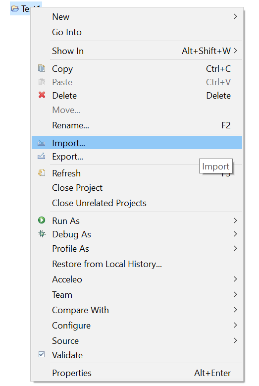
Right-click on the project folder (in this example, the name of the project is "Test1"). You will see several possible options. In that menu select and click "Import...".
This will open a dialogue where different available import options are listed.
Step 3
Open the folder called "AMALTHEA Trace DB" by clicking on cross next to the title. This is shown in the following picture:
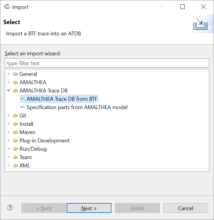
Select the option "AMALTHEA Trace DB from BTF" and click the "Next" button.
Step 4
You are prompted to enter the location of the BTF file you want to import. Click the upper "Browse..." button to navigate your file system and select the "test1.btf" file. If you want to change the target project the ATDB file will be created in, press the lower "Browse..." button and make your choice. If you want the original trace data from the BTF in the data base file, select the option "Persist trace event table". The figure shows the example input:
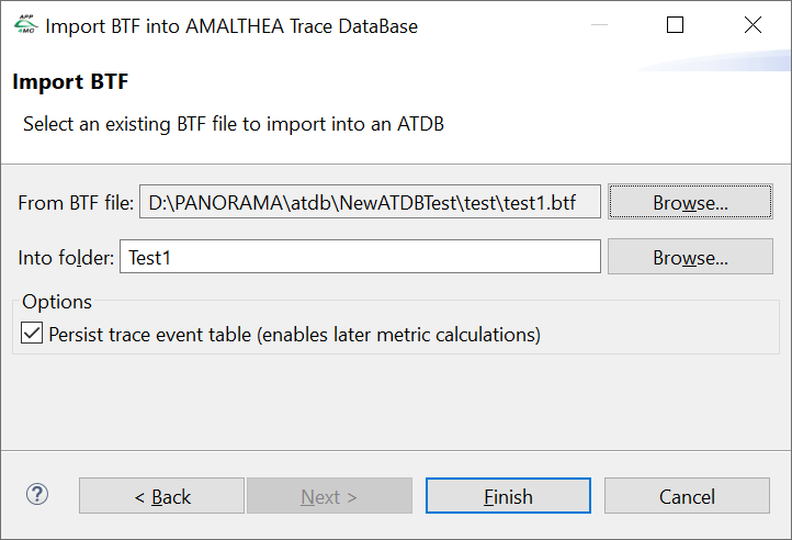
Step 5
After you have made all required inputs, click on "Finish". This will start the import of the database. Once the transformation is done the dialogue will close and the newly created ATDB file is opened in the Metric Viewer. For our example, this is shown in the following figure:
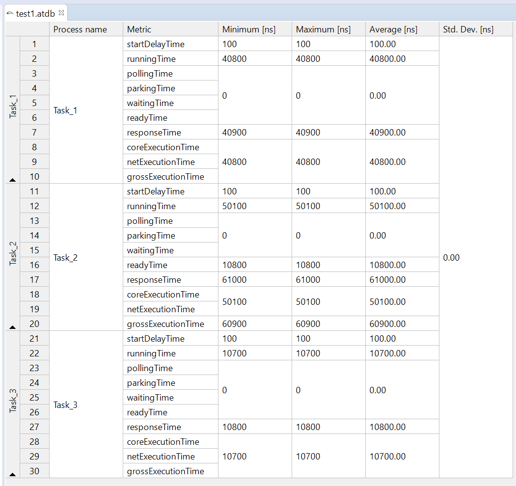
2.4.2 AMALTHEA Specification Parts to ATDB Import Example
This section describes how to use the information contained in an AMALTHEA model to enrich an existing ATDB with the specification parts (events and event chains).
Step 1
Consider the following original AMALTHEA model (called "test1model.amxmi") of which we want to import and analyze the events and event chains in the already existing test1.atdb file.
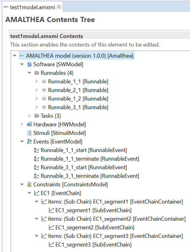
Step 2
Select both files, test1.atdb and test1model.amxmi in the Project Explorer (press and hold Ctrl while clicking on the second file). Right-click on your selection and click "AMALTHEA Specifications -> ATDB" in the contest menu:
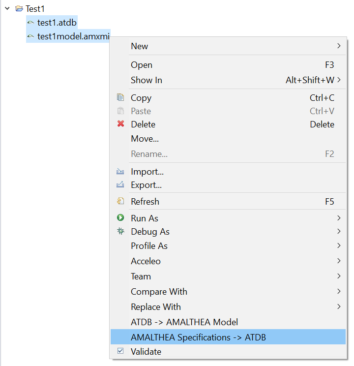
Step 3
This will then create and open the enriched ATDB (which is named after the original amxmi file) in the metric viewer.
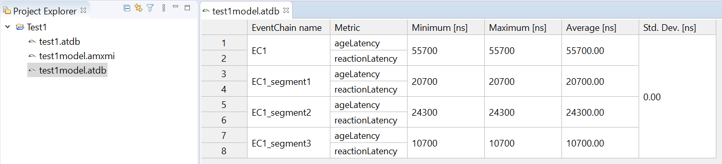
As can be seen in the picture, there is now metric data about the events and event chains from the test1model.amxmi file.
2.4.3 ATDB to AMALTHEA Model Transformation
Here, we describes how to use the information contained within an AMALTHEA Trace Database (ATDB) to create an initial AMALTHEA model from it.
Step 1
Let us assume there is an ATDB file called "test2.atdb" which contains typical atdb data about a trace and some specification parts (events and event chains):
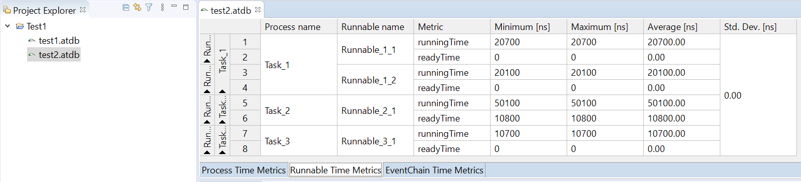
Step 2
We now want to create an AMALTHEA model to start out on an initial simulateable model from the contained trace data. For this right-click on the "test2.atdb" file in the Project Explorer:
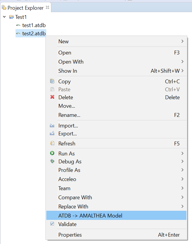
Now, click on "ATDB -> AMALTHEA model".
Step 3
This will create a new AMALTHEA model from the ATDB file (here, called "test2.amxmi". The result will contain all information about the software, hardware, events, and event chains that the original ATDB file provided.
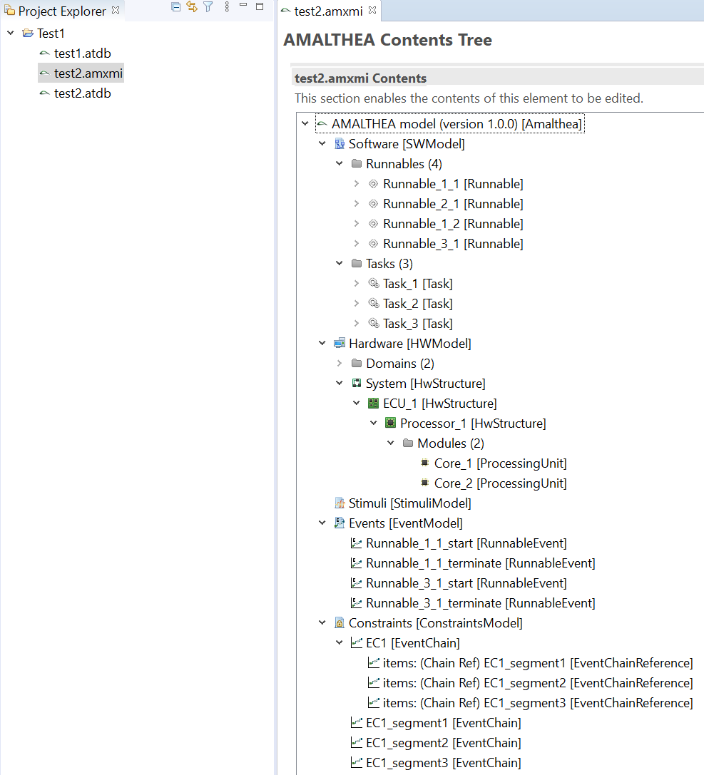
2.5 Editors / Viewers
2.5.1 AMALTHEA Trace Database Metrics Viewer
This is a simple viewer that shows how to access the AMALTHEA trace database.
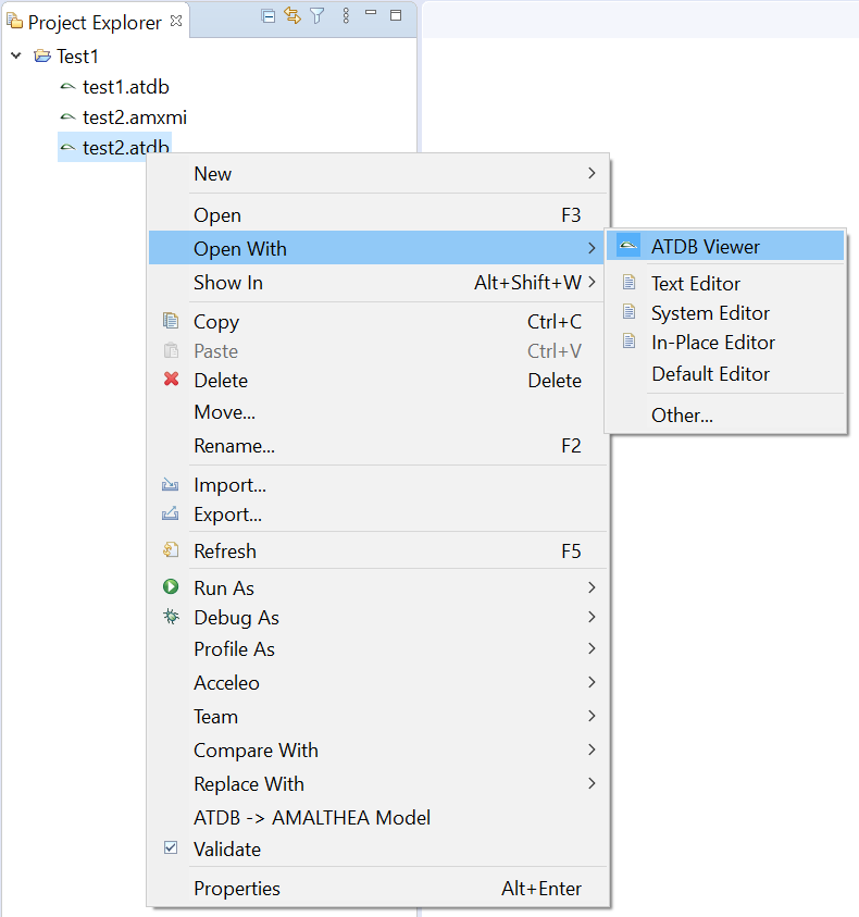
The ATDB metrics viewer displays metrics in three tabs: "Process Time Metrics", "Runnable Time Metrics", and "EventChain Time Metrics". The table in each tab displays various time metrics (depending on what events were actually in the source trace). The time metrics are aggregated, i.e., Minimum, Maximum, Average, and Standard Deviation values of the entity instances are shown. For better navigability you can collapse the metric value rows per entity. The following figure shows the metric table for processes:
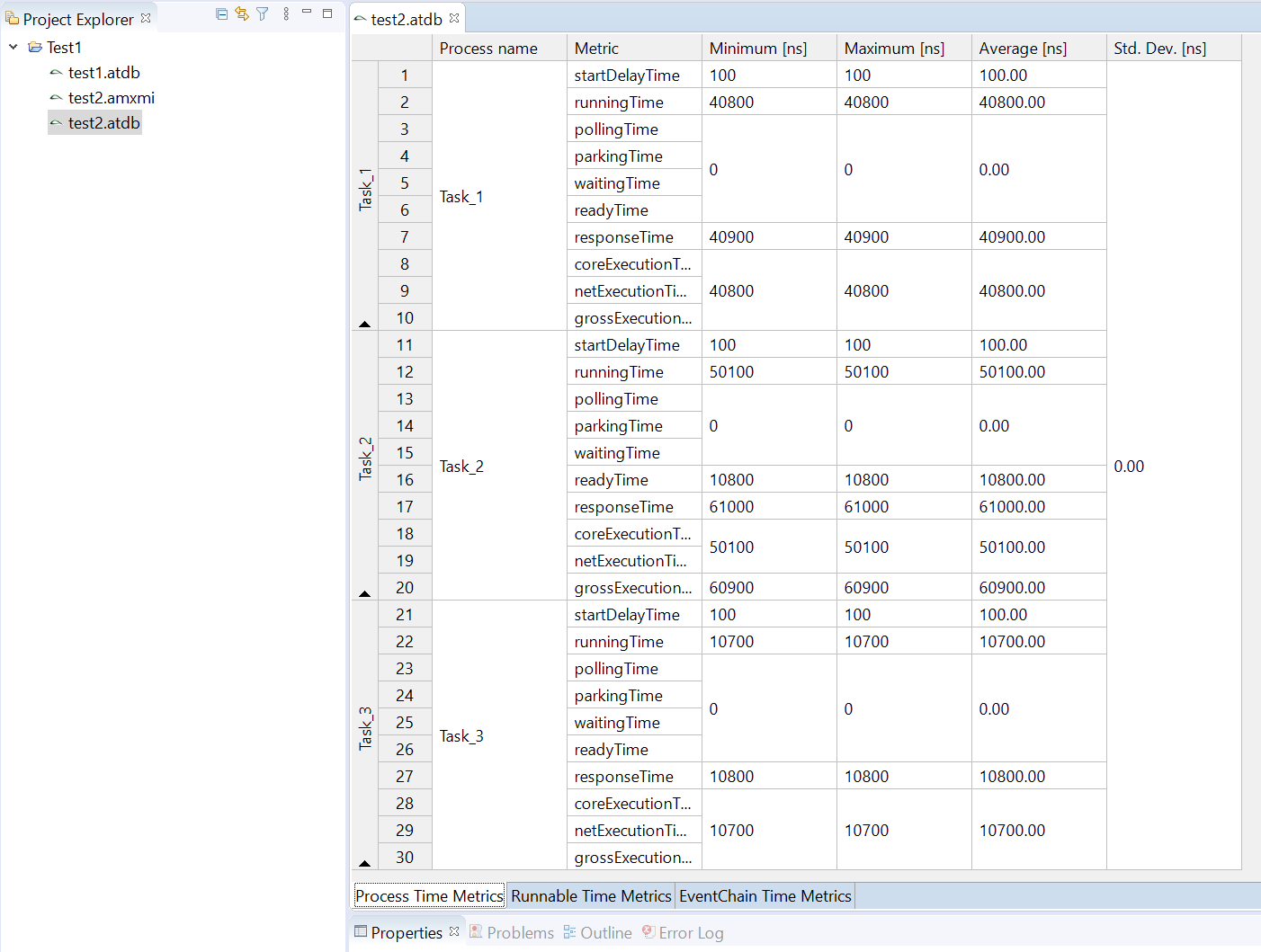
And the next picture shows the same table with the metrics of "Task_1" and "Task_2" collapsed.
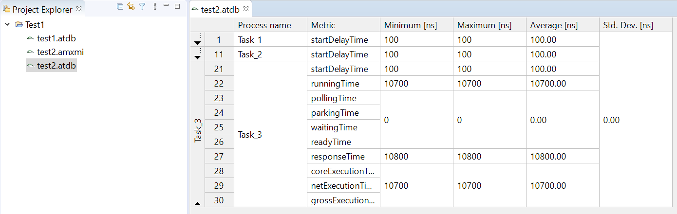
2.6 Model Visualization
2.6.1 Usage of AMALTHEA Model Visualization
The AMALTHEA Visualization can be opened via
-
Window → Show View → Other... → APP4MC → APP4MC Visualizations,
- or via right click on an element and selecting
Open APP4MC Visualization.
Via the context menu it is also possible to open multiple visualization views.
On selecting a model element, the view will render a corresponding visualization. If multiple visualizations are available, the first one will be selected by default, unless the user has selected another visualization before.
The visualization view has 4 entries in the toolbar:
-
Visualization dropdown
The dropdown contains all available visualizations for the current active selection. A click on the image will reload the visualization.
-
Pin visualization
The selection handling will be disabled so the visualization gets not updated on model selection changes.
-
Select model element
Selects the current visualized model element in the model editor. Useful for example if a visualization is pinned and the selection in the model editor changed.
-
View Menu
Contains entries to customize title and supported visualizations of the current view.
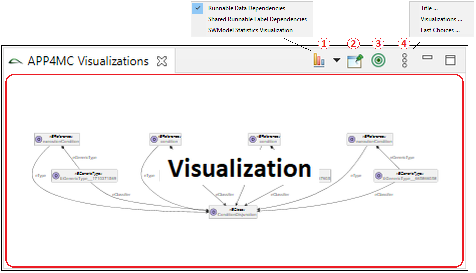
2.6.2 Standard Visualizations
APP4MC comes with a set of default model visualizations to show the options and possibilities the visualization framework provides.
Hardware Model
-
HW Model Block Diagram
This visualization is intended to provide an overview of the described and used hardware within the system.
It uses PlantUML and SVG for rendering. Therefore a Graphviz dot.exe needs to be configured via
Window – Preferences – PlantUML – Path to the dot executable of Graphviz in order to get the result shown.
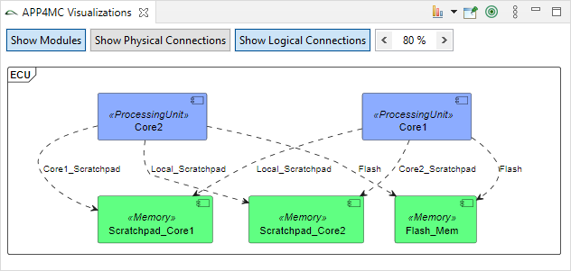
Software Model
-
SWModel Statistics Visualization
This is a simple visualization that shows some statistics on the selected Software Model. It is also a simple example to show how to implement a visualization with JavaFX and some animations.
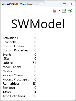
-
Shared Runnable Label Dependencies
This visualization paints all
Runnables and the read/write dependencies on
Labels in a Software Model.
Via the buttons on the left edge you can
Zoom in (+) / Zoom out (-) / Filter (F) the currently visible
Runnables.
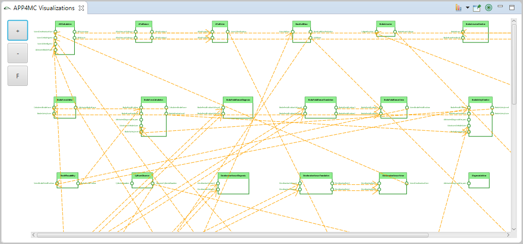
-
Runnable Data Dependencies
The purpose of this small - but
hopefully useful - visualization is to lay out a graph of the
Runnables
in a software model based on there data dependencies.
This means, two runnables are connected by a directed edge if the first
runnable writes a
Label
that is read by the second one.
Furthermore, some parts of the control flow are expressed by edges. The
tool colors the graph in order to make it easier for the user to follow
individual edges.
For the visualization to work properly, the path to Graphviz DOT has
to be set up in the PlantUML preferences. You can access them via
Window > Preferences...
and then opening the PlantUML tab.
The buttons in the top row are used to configure the
visualization.
-
Horizontal Layout:
Toggle between horizontal
(left to right) and vertical (top to bottom) layout of the
graph.
-
Show Labels:
Show read and written labels of the
runnables.
-
Show R/W Dependencies:
Show read/write data
dependencies between runnables. This is independent from the labels
being shown.
-
Show Control Flow:
Show stimuli, inter-process
triggers, and OS events. Also show the sequence of runnables within a
task.
-
Show Tasks:
Group runnables by tasks.
-
Export:
Export the visualization as an image, or
as Graphiz DOT. Supported image formats are PDF, SVG, and
PNG. Output in other formats can be generated by exporting in DOT
format and running Graphviz manually.
-
+ / -:
Zoom in/out.
For performance reasons, the visualization has been limited to models
containing at most 200 runnables. This limitation does not apply to
the export of the graph in DOT format.
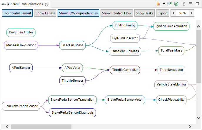
The table below summarizes which elements are visualized. The
following elements are considered:
- Within a Runnable: LabelAccess
- Within a Task:
Group, RunnableCall,
InterProcessTrigger,
WaitEvent,
SetEvent
Other activity items (e.g. ProbabilitySwitch) are simply
ignored. Using them may lead to incomplete results.
| Runnables |
|
| Stimuli |

|
| Tasks |

|
| Data dependencies |

(colored edges)
|
| Runnable sequence in tasks |

|
| Inter-process stimuli, OS events |

|
Runnable
-
LabelAccess View
A simple visualization of a
Runnable and its
Label read/write access. On the left side the
Labels are rendered that are accessed for a read operation. On the right side the
Labels are rendered that are accessed for a write operation.
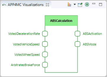
-
Shared Runnable Label Dependencies
Visualization of all selected
Runnables and their relationships based on
Labels. This visualization is an example to verify how to implement a visualization on multi-selection.
Via the buttons on the left edge you can
Zoom in (+) / Zoom out (-) / Filter (F) the currently visible
Runnables.
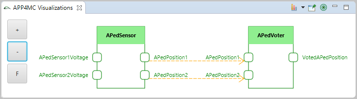
-
Runnable Label Dependencies
This visualization shows the current selected
Runnable and the
Runnables that have a direct dependency via
Labels. On the left side the
Runnables are rendered that
write to
Labels that are read by the selected
Runnable. On the right side the
Runnables are rendered that
read from
Labels that were modified by the selected
Runnable.
Via the buttons on the left edge you can
Zoom in (+) / Zoom out (-) the currently visible
Runnables.
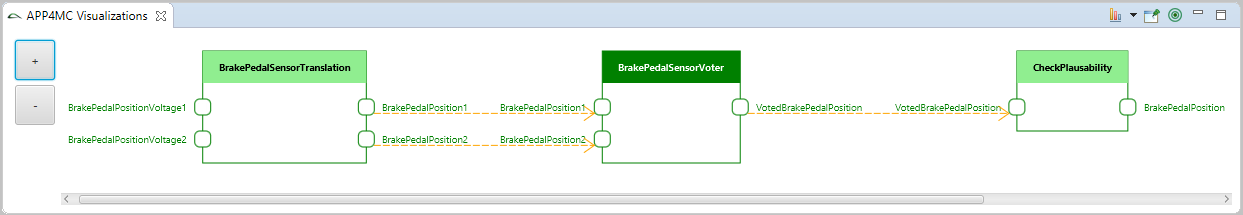
Deviation
-
Probability Density Diagram
This visualization provides probability density diagrams for all subclasses of
- IContinuousValueDeviation
- IDiscreteValueDeviation
- ITimeDeviation
Markers (vertical lines) are shown for lower bound, upper bound and average.
Changed values in the Properties view lead to an update of the diagram.
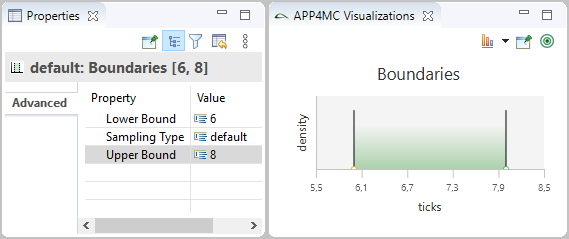
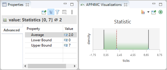
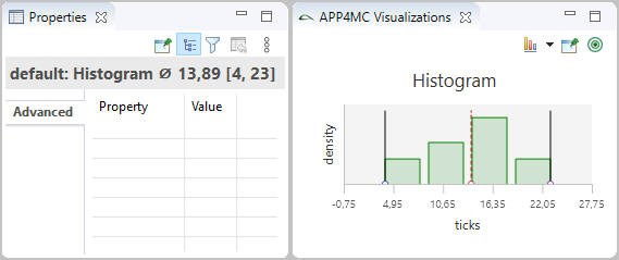
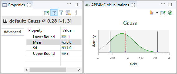
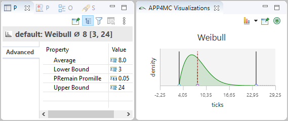
Mapping
-
Scheduler Mapping Table
This visualization shows a (hierarchical) table of schedulers, processing units and processes.
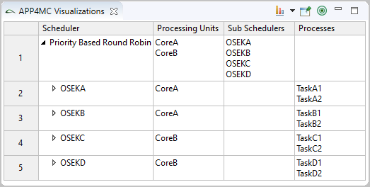
Object References
-
Object References View
This visualization shows objects that refer to the selected object.
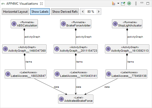
Specific back-references
The visualizations in this section show a simple list of objects that refer to the selected attribute.
A double click on a list item allows to navigate to the corresponding object.
-
Namespace members
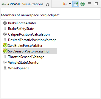
Further visualizations (without screenshot):
Eventchain Map
-
Eventchain Map
This visualization shows the (nested) segments of an event chain.
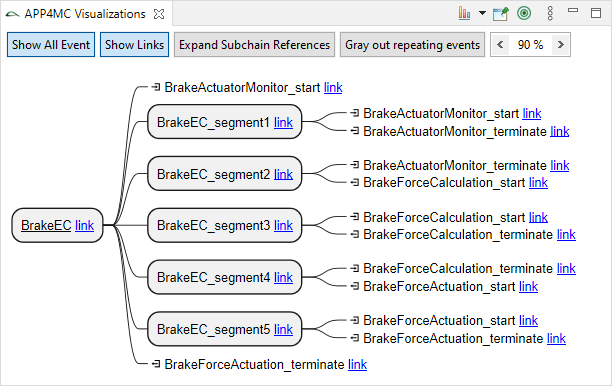
2.7 Model Validation
2.7.1 Usage of AMALTHEA Model Validation
The AMALTHEA model validation can be triggered by clicking on the "Validate" button of the Amalthea editor.
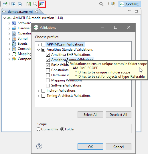
The dialog shows a list of profiles allowing the selection of specific validations.
The validation is either applied to all elements of the model (default: folder scope) or only to the elements of the current file.
If an error is found, it is shown in the Problems view of Eclipse. A simple double click on the error will lead you to the affected elements in the AMALTHEA model. The validation distinguishes between three error types:
errors,
warnings and
info.
2.7.2 Included Validations
Amalthea Standard Validations
org.eclipse.app4mc.amalthea.validations.standard.AmaltheaProfile
Amalthea Standard Validations
Standard validations for AMALTHEA models to ensure data consistency.
- Profiles:
-
org.eclipse.app4mc.amalthea.validations.standard.BasicProfile
-
org.eclipse.app4mc.amalthea.validations.standard.ConstraintsProfile
-
org.eclipse.app4mc.amalthea.validations.standard.EMFProfile
-
org.eclipse.app4mc.amalthea.validations.standard.HardwareProfile
-
org.eclipse.app4mc.amalthea.validations.standard.MappingProfile
-
org.eclipse.app4mc.amalthea.validations.standard.OSProfile
-
org.eclipse.app4mc.amalthea.validations.standard.SoftwareProfile
org.eclipse.app4mc.amalthea.validations.standard.BasicProfile
Basic Validations
- Validations:
- AM-Basic-Counter (ERROR – Counter)
- The offset value of a counter must not be negative
- AM-Basic-Data-Size (ERROR – DataSize)
- Some data sizes have to fulfill the condition >0 or >=0
- AM-Basic-Frequency (ERROR – Frequency)
- Some frequencies have to fulfill the condition >0
- AM-Basic-Quantity (ERROR – Quantity)
- Quantity unit has to be set (
undefined is an error)
- AM-Basic-Time-Range (ERROR – Time)
- Some time ranges has to fulfill the condition >0 or >=0
- AM-Basic-CustomProperty-Key (WARNING – IAnnotatable)
- Custom property keys have to be unique
org.eclipse.app4mc.amalthea.validations.standard.ConstraintsProfile
Constraints Validations
- Validations:
- AM-Constraints-EventChain (ERROR – AbstractEventChain)
- Stimulus and response shall not reference the same event
- The response of the last segment has to be the same as the response of the event chain
- The stimulus of other segments have to be equal to the response of the previous segment
- The stimulus of the first segment has to be the same as the stimulus of the event chain
org.eclipse.app4mc.amalthea.validations.standard.EMFProfile
Amalthea EMF Validations
Standard EMF validations for AMALTHEA models (generated).
- Validations:
- AM-EMF-INTRINSIC (UNDEFINED – EObject)
- AMALTHEA invariants (generated)
- EMF extended metadata constraints (generated)
org.eclipse.app4mc.amalthea.validations.standard.HardwareProfile
Hardware Validations
- Validations:
- AM-HW-AccessPath (ERROR – HwAccessPath)
- HwAccessPath elements must be consistent
- HwAccessPath ranges and memory size must be consistent
- AM-HW-Connection (ERROR – HwConnection)
- HwConnections must be linked to HwPorts of the same Interface
- HwConnections must refer to two HwPorts
- AM-HW-Definition (ERROR – HwDefinition)
- Only one feature of a category can be referred
- AM-HW-Port (ERROR – HwPort)
- A HwPort can only have one (non internal) HwConnection
- AM-HW-Structure (ERROR – HwStructure)
- Connections must only refer to contained HwPorts
- Delegated connections always connect HwPorts of the same type
- Inner connections always need one Initiator and one Responder HwPort
- AM-HW-Module-Definition (WARNING – HwModule)
- Cache definition must be set
- ConnectionHandler definition must be set
- Memory definition must be set
- ProcessingUnit definition must be set
- AM-HW-Port-BitWidth (WARNING – HwPort)
- Bitwidth should be greater than zero
- AM-HW-Port-Definition (WARNING – HwPort)
- PortInterface must be set
- PortType must be set
org.eclipse.app4mc.amalthea.validations.standard.MappingProfile
Mapping Validations
- Validations:
- AM-Mapping-ISR-Scheduler (WARNING – ISR)
- An ISR should have an allocation to an interrupt controller
- AM-Mapping-Scheduler-Allocation-Hierarchy (WARNING – SchedulerAllocation)
- A child scheduler should only be responsible for a subset of processing units of its ancestors
- AM-Mapping-Scheduler-Allocation-Top-Level-Responsibility (WARNING – MappingModel)
- A processing unit should have at most one top level task scheduler and one interrupt controller responsible for it
- AM-Mapping-Scheduler-ProcessingUnit (WARNING – Scheduler)
- A top level scheduler should be responsible for at least one processing unit
- AM-Mapping-Task-Scheduler (WARNING – Task)
- A task should have an allocation to a task scheduler
org.eclipse.app4mc.amalthea.validations.standard.OSProfile
OS Validations
- Validations:
- AM-OS-Mandatory-Scheduling-Parameters-Set (ERROR – Scheduler)
- Mandatory scheduling parameters must be set
- AM-OS-Scheduling-Parameter-Value-Number-Matches-Defined-Multiplicity (ERROR – Entry)
- The number of values of the specified scheduling parameter must match the defined multiplicity in the scheduling parameter definition
- AM-OS-Scheduling-Parameter-Value-Type-Matches-Defined-Type (ERROR – Entry)
- The type of the specified scheduling parameter must match the type defined in the scheduling parameter definition
- AM-OS-Semaphore-Properties-Conform-Type (ERROR – Semaphore)
- Semaphore properties conform to semaphore type
- AM-OS-Scheduling-Parameter-Empty-Overriden-Value (WARNING – Entry)
- There should be a value if a default value of a scheduling parameter is overridden
- AM-OS-Standard-Scheduler-Definition-Conformance (WARNING – SchedulerDefinition)
- Standard schedulers with their parameters should be modeled as defined by the APP4MC standard scheduler library
- AM-OS-Standard-Scheduling-Parameter-Definition-Conformance (WARNING – SchedulingParameterDefinition)
- Scheduling parameter definition that are used in a standard scheduler should conform to the parameters defined by the APP4MC standard scheduler library
org.eclipse.app4mc.amalthea.validations.standard.SoftwareProfile
Software Validations
- Validations:
- AM-SW-CallArgument (ERROR – CallArgument)
- The referred runnable must contain the referred parameter
- AM-SW-DataDependency (ERROR – DataDependency)
- A data dependency can only be defined for specific types of label accesses, parameters and call arguments
- A data dependency can only refer to specific types of parameters and call arguments
- AM-SW-Group (ERROR – Group)
- The uninterruptible group must not contain nested groups
- AM-SW-Semaphore-Access (ERROR – SemaphoreAccess)
- Waiting behaviour must be 'active' for spinlock semaphore access
APP4MC.sim Validations
org.eclipse.app4mc.amalthea.validations.sim.App4mcSimProfile
APP4MC.sim Validations
Validations for AMALTHEA models used in a APP4MC.sim simulation.
- Profiles:
-
org.eclipse.app4mc.amalthea.validations.sim.SimBasicProfile
-
org.eclipse.app4mc.amalthea.validations.sim.SimHardwareProfile
-
org.eclipse.app4mc.amalthea.validations.sim.SimMappingProfile
-
org.eclipse.app4mc.amalthea.validations.sim.SimOsProfile
-
org.eclipse.app4mc.amalthea.validations.sim.SimSoftwareProfile
-
org.eclipse.app4mc.amalthea.validations.standard.AmaltheaProfile
org.eclipse.app4mc.amalthea.validations.sim.SimBasicProfile
Basic Validations (APP4MC.sim)
- Validations:
- Sim-Basic-Identifiers (ERROR – IReferable)
- All names of IReferable objects must be valid C++ identifier names
- TA-Basic-ContinuousValueGaussDistribution-mean (ERROR – ContinuousValueGaussDistribution)
- Mean must not be greater than the upper bound
- Mean must not be less than the lower bound
- TA-Basic-DiscreteValueGaussDistribution-mean (ERROR – DiscreteValueGaussDistribution)
- Mean must not be greater than the upper bound
- Mean must not be less than the lower bound
- TA-Basic-TimeGaussDistribution-mean (ERROR – TimeGaussDistribution)
- Mean must not be greater than the upper bound
- Mean must not be less than the lower bound
- Sim-supported-model-elements (WARNING – EObject)
- Checks that the model elements are supported in APP4MC.sim
org.eclipse.app4mc.amalthea.validations.sim.SimHardwareProfile
Hardware Validations (APP4MC.sim)
- Validations:
- Inchron-HWModule-MissingClockReference (ERROR – HwModule)
- HW Module must have 'Frequency Domain' reference
- Sim-HW-ProcessingUnit (ERROR – ProcessingUnit)
- ProcessingUnit definition must be set
- Sim-HW-AccessElement (WARNING – HwAccessElement)
- Either hwAccessPath must be set or at least one of read latency and datarate must be set. Either hwAccessPath must be set or at least one of write latency and datarate must be set.
- Sim-HW-Connection (WARNING – HwConnection)
- Either read latency or data rate or both must be set. Either write latency or data rate or both must be set.
- Sim-HW-MemoryDefinition (WARNING – MemoryDefinition)
- Either access latency or datarate (or both) must be set
org.eclipse.app4mc.amalthea.validations.sim.SimMappingProfile
Mapping Validations (APP4MC.sim)
- Validations:
- AM-Mapping-ISR-Scheduler (ERROR – ISR)
- An ISR should have an allocation to an interrupt controller
- AM-Mapping-Scheduler-Allocation-Hierarchy (ERROR – SchedulerAllocation)
- A child scheduler should only be responsible for a subset of processing units of its ancestors
- AM-Mapping-Scheduler-Allocation-Top-Level-Responsibility (ERROR – MappingModel)
- A processing unit should have at most one top level task scheduler and one interrupt controller responsible for it
- AM-Mapping-Scheduler-ProcessingUnit (ERROR – Scheduler)
- A top level scheduler should be responsible for at least one processing unit
- AM-Mapping-Task-Scheduler (ERROR – Task)
- A task should have an allocation to a task scheduler
- Sim-Mapping-SchedulerAllocation (WARNING – SchedulerAllocation)
- Executing processing unit must be set
org.eclipse.app4mc.amalthea.validations.sim.SimOsProfile
OS model Validations (APP4MC.sim)
- Validations:
- AM-OS-Mandatory-Scheduling-Parameters-Set (ERROR – Scheduler)
- Mandatory scheduling parameters must be set
- AM-OS-Scheduling-Parameter-Value-Number-Matches-Defined-Multiplicity (ERROR – Entry)
- The number of values of the specified scheduling parameter must match the defined multiplicity in the scheduling parameter definition
- AM-OS-Scheduling-Parameter-Value-Type-Matches-Defined-Type (ERROR – Entry)
- The type of the specified scheduling parameter must match the type defined in the scheduling parameter definition
- AM-OS-Standard-Scheduler-Definition-Conformance (ERROR – SchedulerDefinition)
- Standard schedulers with their parameters should be modeled as defined by the APP4MC standard scheduler library
- AM-OS-Standard-Scheduling-Parameter-Definition-Conformance (ERROR – SchedulingParameterDefinition)
- Scheduling parameter definition that are used in a standard scheduler should conform to the parameters defined by the APP4MC standard scheduler library
- Inchron-OS-PU-Allocation-MustBeDisjunct (INFO – OperatingSystem)
- OS Scheduler to core mapping must be distinct
org.eclipse.app4mc.amalthea.validations.sim.SimSoftwareProfile
Software Validations (APP4MC.sim)
- Validations:
- Sim-Software-AbstractMemoryElementIsMapped (ERROR – Label)
- Checks if label is mapped to a memory node
- Sim-Software-AbstractMemoryElementIsMapped (ERROR – LabelAccess)
- Checks if label access type is set
- Sim-Software-AbstractMemoryElementIsMapped (ERROR – ModeLabelAccess)
- Checks if modeLabel access type is valid
- Sim-Software-AbstractMemoryElementIsMapped (ERROR – Channel)
- Checks if channel is mapped to a Memory
- Sim-Software-ChannelAccessFeasibility (ERROR – ChannelAccess)
- Checks if a channel access can be performed from certain runnable
- Sim-Software-ChannelElements (ERROR – ChannelAccess)
- Checks if channel access's property elements is greater 0
- Sim-Software-LabelAccessFeasibility (ERROR – LabelAccess)
- Checks if a label access can be performed from certain runnable
- Sim-Software-Process (ERROR – Process)
- At least one stimulus must be set
- Inchron-SW-Task-MustHaveActivityGraph (WARNING – Task)
- Task must have atleast one ActivityGraph
- Sim-Software-AbstractMemoryElementIsMapped (WARNING – ModeLabel)
- Checks if modeLabel is mapped to a Memory
- Sim-Software-ModeLabelAccessFeasibility (WARNING – ModeLabelAccess)
- Checks if a modeLabel access can be performed from certain runnable
- TA-Software-ModeConditionConjunctionAlwaysFalse (WARNING – ConditionConjunction)
- TA-Software-ModeConditionDisjunctionAlwaysTrue (WARNING – ConditionDisjunction)
- Inchron-SW-Runnable-MustHaveActivityGraph (INFO – Runnable)
- Runnable must have at least one ActivityGraph
Timing Architects Validations
org.eclipse.app4mc.amalthea.validations.ta.TimingArchitectsProfile
Timing Architects Validations
Validations for AMALTHEA models used in a Timing Architects Simulation.
- Validations:
- TA-Misc-Semaphore (ERROR – Semaphore)
- Initial value must not be negative
- Max value must be positive
- Max value must not be smaller than the initial value
- Profiles:
-
org.eclipse.app4mc.amalthea.validations.standard.AmaltheaProfile
-
org.eclipse.app4mc.amalthea.validations.ta.TABasicProfile
-
org.eclipse.app4mc.amalthea.validations.ta.TAConstraintsProfile
-
org.eclipse.app4mc.amalthea.validations.ta.TAHardwareProfile
-
org.eclipse.app4mc.amalthea.validations.ta.TASoftwareProfile
-
org.eclipse.app4mc.amalthea.validations.ta.TAStimuliProfile
org.eclipse.app4mc.amalthea.validations.ta.TABasicProfile
Basic Validations (Timing Architects)
- Validations:
- TA-Basic-ContinuousValueGaussDistribution-mean (ERROR – ContinuousValueGaussDistribution)
- Mean must not be greater than the upper bound
- Mean must not be less than the lower bound
- TA-Basic-DiscreteValueGaussDistribution-mean (ERROR – DiscreteValueGaussDistribution)
- Mean must not be greater than the upper bound
- Mean must not be less than the lower bound
- TA-Basic-TimeGaussDistribution-mean (ERROR – TimeGaussDistribution)
- Mean must not be greater than the upper bound
- Mean must not be less than the lower bound
org.eclipse.app4mc.amalthea.validations.ta.TAConstraintsProfile
Constraints Validations (Timing Architects)
- Validations:
- TA-Constraints-DataAgeTime (ERROR – DataAgeTime)
- Maximum time must not be smaller than minimum time
- TA-Constraints-DelayConstraint (ERROR – DelayConstraint)
- Upper bound must not be smaller than lower bound
- TA-Constraints-ECLConstraint (ERROR – EventChainLatencyConstraint)
- Maximum must not be smaller than minimum
- TA-Constraints-RTLimitMustBePositive (ERROR – TimeRequirementLimit)
- Response time must be positive
- TA-Constraints-RepetitionConstraint (ERROR – RepetitionConstraint)
- Upper bound must not be smaller than lower bound
org.eclipse.app4mc.amalthea.validations.ta.TAHardwareProfile
Hardware Validations (Timing Architects)
- Validations:
- TA-Hardware-HWFIPCMustBePositive (ERROR – HwFeature)
- IPC (instructions per cycle) must be positive
- TA-Hardware-PUDIPCMissing (INFO – ProcessingUnitDefinition)
- IPC (instructions per cycle) should be set, otherwise default (1.0) will be assumed
- Only one IPC HwFeature should be specified for a processing unit definition
org.eclipse.app4mc.amalthea.validations.ta.TASoftwareProfile
Software Validations (Timing Architects)
- Validations:
- TA-Software-RunnableCall (ERROR – RunnableCall)
- TA-Software-ServerCall (ERROR – ServerCall)
- TA-Stimuli-ArrivalCurveStimulus (ERROR – OsEvent)
- TA-Software-ModeConditionConjunctionAlwaysFalse (WARNING – ConditionConjunction)
- TA-Software-ModeConditionDisjunctionAlwaysTrue (WARNING – ConditionDisjunction)
org.eclipse.app4mc.amalthea.validations.ta.TAStimuliProfile
Stimuli Validations (Timing Architects)
- Validations:
- TA-Stimuli-VariableRateStimulusScenario (ERROR – VariableRateStimulus)
Inchron Validations
org.eclipse.app4mc.amalthea.validations.inchron.InchronProfile
Inchron Validations
Validation for Amalthea models used in Inchron Toolsuite
- Profiles:
-
org.eclipse.app4mc.amalthea.validations.inchron.InchronConstraintsProfile
-
org.eclipse.app4mc.amalthea.validations.inchron.InchronHWProfile
-
org.eclipse.app4mc.amalthea.validations.inchron.InchronOsProfile
-
org.eclipse.app4mc.amalthea.validations.inchron.InchronSoftwareProfile
-
org.eclipse.app4mc.amalthea.validations.inchron.InchronStimuliProfile
-
org.eclipse.app4mc.amalthea.validations.standard.AmaltheaProfile
org.eclipse.app4mc.amalthea.validations.inchron.InchronConstraintsProfile
Constraints Validations (INCHRON)
- Validations:
- Inchron-Constraints-LoadRequirementMissingResource (ERROR – CPUPercentageRequirementLimit)
- CPU load requirement must have hardware context
org.eclipse.app4mc.amalthea.validations.inchron.InchronHWProfile
Hardware Validations (INCHRON)
- Validations:
- AM-HW-Port-BitWidth (ERROR – HwPort)
- Bitwidth should be greater than zero
- Inchron-HW-Memory-PortTypeResponder (ERROR – Memory)
- HW ports of memory should be of type responder
- Inchron-HW-PU-PortTypeInitiator (ERROR – ProcessingUnit)
- HW ports of processing Unit should be of type initiator
- Inchron-HWModule-InconsistentPortWidths (ERROR – HwModule)
- HW Module cannot have ports with unequal bitwidth
- Inchron-HWModule-MissingClockReference (ERROR – HwModule)
- HW Module must have 'Frequency Domain' reference
- Profiles:
-
org.eclipse.app4mc.amalthea.validations.standard.HardwareProfile
org.eclipse.app4mc.amalthea.validations.inchron.InchronOsProfile
Operating Systems Validations (INCHRON)
- Validations:
- Inchron-OS-PU-Allocation-MustBeDisjunct (ERROR – OperatingSystem)
- OS Scheduler to core mapping must be distinct
- Inchron-OS-Scheduler-Allocation-DifferentCPU (ERROR – Scheduler)
- OS Task scheduler should not be allocated to more than one HwStructure
- Inchron-OS-UserSpecificSchedulerCheck (ERROR – Amalthea)
- User specific task scheduler needs at least one task allocation
org.eclipse.app4mc.amalthea.validations.inchron.InchronSoftwareProfile
Software Validations (INCHRON)
- Validations:
- Inchron-SW-Runnable-MustHaveActivityGraph (ERROR – Runnable)
- Runnable must have at least one ActivityGraph
- Inchron-SW-Runnable-NotAllocated-DifferentOS (ERROR – Runnable)
- Runnable cannot be scheduled by more than one OS
- Inchron-SW-RunnableAllocation-Present (ERROR – RunnableAllocation)
- Runnable allocation is not supported
- Inchron-SW-Task-EnforcedMigrationCheck (ERROR – Task)
- Invalid Enforced Migration of a task to a task Scheduler
- Inchron-SW-Task-MustHaveActivityGraph (ERROR – Task)
- Task must have atleast one ActivityGraph
- Inchron-SW-Task-NotAllocated-DifferentSchedulers (ERROR – Task)
- Task cannot be scheduled by more than one OS
- Profiles:
-
org.eclipse.app4mc.amalthea.validations.standard.SoftwareProfile
org.eclipse.app4mc.amalthea.validations.inchron.InchronStimuliProfile
Stimuli Validations (INCHRON)
- Validations:
- Inchron-Stimuli-TypeCheck (ERROR – Stimulus)
- Unsupported stimuli types
2.8 Model Migration
2.8.1 AMALTHEA Model Migration
Why model migration is required ?
EMF based models are the instances of ECORE meta model (which is updated for each release).
As there is a tight dependency between model instance and the corresponding meta model, old EMF models can not be loaded with the newer release of meta model.
Example : Due to the change in the namespace of the meta model, loading of model files from prior versions would fail with the latest version
This problem can be solved by explicitly migrating the model files from the prior versions to be compatible to the latest meta model version
AMALTHEA model migration
As described above, same scenario is also applicable for AMALTHEA models as they are instances of EMF based AMALTHEA ECORE meta model.
For each release of AMALTHEA there will be changes in the meta model contents, due to this it is not possible to load models built from previous releases of AMALTHEA into latest tool distribution.
Model Migration functionality is part of this distribution, using this feature it is possible to convert models from previous APP4MC releases to the ones which are compatible to the next versions of AMALTHEA meta model.
Only forward migration of models is supported by Model Migration functionality of AMALTHEA
Warning:
Migration of Amalthea models belonging to legacy versions (ITEA "1.0.3, 1.1.0, 1.1.1") is no longer supported.
If there are Amalthea models belonging to legacy versions, use APP4MC version 0.9.2 (or older) and convert the models into a APP4MC model version. These models can still be used as input for model migration.
2.8.2 Supported versions for model Migration
Model migration functionality provides a possibility to migrate the models (
created from previous releases of AMALTHEA ) to the latest versions.
Only forward migration is supported.
AMALTHEA meta model versions information
- Oldest version to migrate is
APP4MC 0.7.0
Beginning with that version, the AMALTHEA meta model is a part of the official Eclipse project
APP4MC.
Model migration
As described above, only forward migration is supported by the AMALTHEA model migration utility.
Model migration utility migrates the specified model sequentially to the next versions (step by step) till expected version is reached.
Hint for APP4MC 0.9.3 and newer:
Migration of Amalthea models belonging to legacy versions (ITEA "1.0.3, 1.1.0, 1.1.1") is no longer supported.
Below figure represents the steps involved in the migration of model from 0.7.0 version to APP4MC 0.8.1 version:
2.8.3 Pre-requisites for AMALTHEA model migration
VM arguments
Default max heap memory (Xmx) used by the APP4MC distribution is 2 GB. In case of migrating huge models, it is recommended to increase this memory to 4 GB before invocation of "AMALTHEA Model Migration" feature
Follow the below steps to increase the heap memory setting of APP4MC :
- Open
app4mc.ini file (
present in the location where APP4MC is installed) and change the parameter -Xmx from 2g to 4g. (
Note: In case if APP4MC plugins are integrated inside custom eclipse application, then corresponding <application_name>.ini file -Xmx parameter should be updated as specified below
)
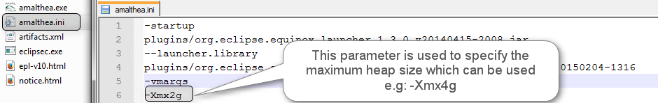
Linked files in eclipse project (virtual files)
In case you want to have linked files in eclipse project, during the drag and drop of the files select
"Link to files" option in
File Operation
dialog and uncheck
create link locations relative to
option
2.8.4 How to invoke AMALTHEA model migration
Simple migration
An attempt to open an older model file in the model editor will show the following dialog.
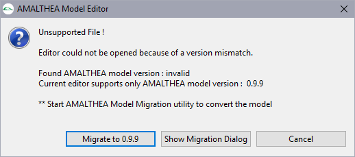
The default button will simply migrate the selected file ...
- provided it doesn't have any references (only allowing single file migration)
- the original file is renamed (the version string is added, e.g. "model_0.9.2.amxmi")
- a log file with the current date is created (e.g. "ModelMigration__2019-07-30_15_43_44.log")
Migration dialog
AMALTHEA model migration utility is developed as a eclipse plugin and it is part of APP4MC distribution
Model migration utility can be invoked by selecting the required models to be migrated in the UI and specifying the target AMALTHEA version to which models should be migrated
Step 1: Selection of AMALTHEA models
Possible selections are:
- a single .amxmi file
- a folder that contains at least one .amxmi file
- a project that contains at least one .amxmi file
Step 2: Opening AMALTHEA Model Migration dialog and configuring migration inputs
On click of AMALTHEA Model Migration action, the following Model Migration dialog is opened:
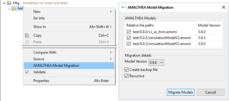
Model Migration dialog consists of following information:
- Selected AMALTHEA model files: These are the models which are included in the selection
Note:
The check box "recursive" allows to include the contents of subfolders
- Input model versions are displayed in the second column of the table
Note:
In case of different AMALTHEA model versions in one folder, a warning will be shown.
- Output model version : This is the AMALTHEA model version to which the selected models files should be migrated to
- If the check box "Create backup file" is checked then a backup file with the same name suffix as in "Simple migration" is created before the migration. Otherwise the migration will be executed in place.
Step 3: Model migration
Once the required parameters are configured in the model migration dialog, click on "Migrate Models" button in the dialog to invoke migration.
The result of the migration will be shown in a new dialog:
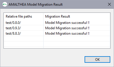
Additionally a log file with the current date is created next to the migrated files (e.g. "ModelMigration__2019-07-30_15_43_44.log").
2.8.5 Additional details
For details regarding the below topics, refer to the corresponding links:
-
How model elements are migrated across various versions ?
-
How to update max heap memory used by the application ?
3 Data Models
3.1 Model Overview
The AMALTHEA data models are related to the activities in a typical design flow. The focus is on design, implementation and optimization of software for multicore systems. The data exchange between the activities is supported by the two main models of AMALTHEA, the System-Model and the Trace-Model.
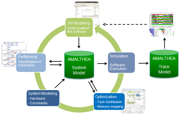
Modeling
The behavior of a component or system is often defined in the form of block diagrams or state charts. Dynamical behavior can also be formalized by differential equations that describe how the state of a system changes over time. Modeling tools like Matlab/Simulink, ASCET or Yakindu allow to simulate the model and to generate software descriptions and implementation.
Partitioning
Based on the description of the software behavior (e.g. label accesses, synchronization, ...) this step identifies software units that can be executed in parallel.
System Modeling
The structure of the hardware (e.g. cores, memory sizes, ...) and system constraints are added to the model.
The constraints are limiting the possible results of the next step.
Optimization
The activity of assigning executable software units to the cores and mapping data and instructions to memory sections. This step can be done manually or supported by a tool that optimizes the partitioning based on information about the software behavior (e.g. data dependencies, required synchronization, etc.).
Simulation / Software Execution
In this step model-based simulation tools evaluate the timing behavior of the software.
Typically these types of high level simulations are based on the hardware and software description of the system.
Low level simulators (e.g. instruction set simulators) or real hardware can be used to execute existing software.
The resulting traces provide additional data that is the basis for a more detailed analysis.
A simplified picture shows the main purpose of the models.
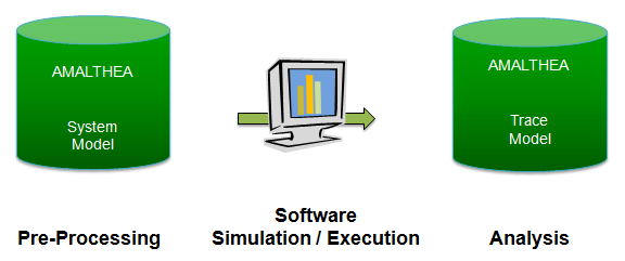
The open AMALTHEA models allow custom tooling, interoperability of tools and the combination of different simulation or execution environments.
3.1.1 AMALTHEA System Model
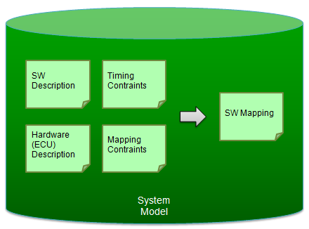
The System Model contains:
Hardware / ECU Description
Hardware abstraction that includes general information about the hardware. Examples are: Number of cores, features of the cores, available memory, access times (from core x to memory y), etc.
SW Description
The description contains information about the static or dynamic behavior the software. This includes: tasks, software components, interfaces, variables, types, etc. It is also possible to describe the characteristics of software functions like the access to variables (read, write, frequency) or the calls to service routines (call tree).
Timing Constraints
Timing Constraints like End-to-End Delay, Latency and Synchronization can be formally written in the "TIMMO Timing Augmented Description Language" (TADL). They are derived from timing requirements or control theory.
Mapping Constraints
The different cores of a typical embedded multicore ECU have different features. For optimal performance it is necessary to restrict the assignment of some software functions to e.g. cores with fastest I/O connections or the maximum clock rate. For safety reasons it is required that some functions are located on specific cores that e.g. can run in lock step mode. Constraints like this are represented in this sub model.
SW Mapping
All information about the assignment of software units (e.g. tasks or runnables) to the cores and about the mapping of data and instructions to memory sections.
3.1.2 AMALTHEA Trace Model
There is no specific EMF data model to describe event traces. The relevant events and their states are represented in the Event Model. In addition special trace formats for multicore have been specified in the AMALTHEA project and a Trace Database has been implemented. This database stores traces in a way that allows fast retrieval of the information (see the Developer Guide for a detailed description of the database structure).
3.1.3 Structure of the model
The definition of the AMALTHEA data model follows some basic principles:
- The model is defined in one package to simplify the handling (e.g. allow opposite references).
- Different aspects are addressed in different logical sub models.
- Existing EMF models from other Eclipse projects are reused and referenced instead of creating own definitions.
- References are based on unique names within the same type of element.
We also try to use ticks wherever possible instead of direct time information. This has advantages in a multi-core environment, as the cores could have different clock frequencies.
The following figure shows the different logical parts of the AMALTHEA data model and how they are referencing each other. The central AMALTHEA model and common model that contains reusable elements are drawn without connections in this diagram.
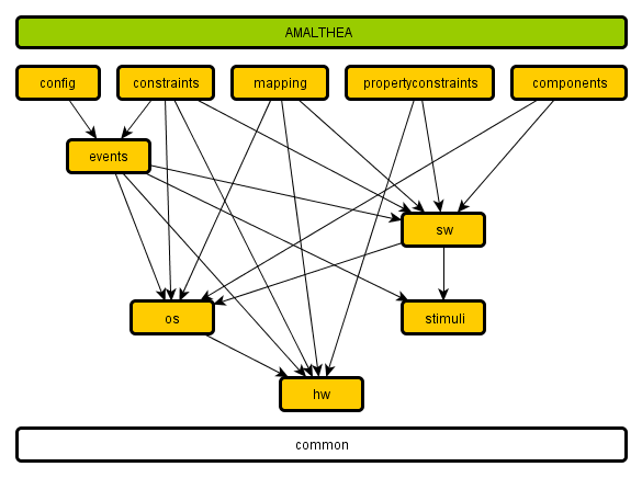
3.2 Model Basics
The following classes are used all over the Amalthea model to define specific attributes of the model classes.
3.2.1 Custom Properties
The
CustomProperty element is used to define own properties that are not (yet) available in AMALTHEA. If there is the need to extend an element or to store tool information related to processing steps,
CustomProperties can be used to store this type of information. It also provides the possibility to work with prototypical approaches that later (if established and more stable) can be integrated in the standard model.
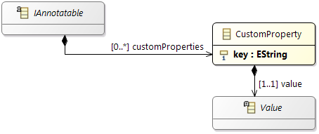
The elements are stored in a
HashMap. The values can be of different types as shown in the structure picture, like String, Integer, Boolean...
In addition a
ReferenceObject is available to store own references to other
EObject elements.
The
ListObject can be used to store multi-valued custom properties and the
MapObject allows nested entries.
3.2.2 Time (and Time Unit)
The AMALTHEA data model includes a common element to describe time ranges in an easy way, the
Time element. The
Time class in general allows to define negative time values. If only positive values are expected the AMALTHEA validation will show a warning.
The
Time element can be contained by any other element for specifying attributes to store time information.
Time units are needed to describe different timing behavior and requirements, like deadlines or offsets of components.
To support different time ranges, especially different time units, AMALTHEA predefines these types like seconds, milli-seconds, micro-seconds, nano-seconds or pico-seconds.
3.2.3 Frequency (and Frequency Unit)
3.2.4 Data Size (and Data Size Unit)
The
DataSize (and
DataRate) definition contains units and prefixes
- according to the SI Standard
- for binary multiples
| International System of Units (SI) |
Prefixes for binary multiples |
|
Name
|
Prefix
|
Factor
|
| kilo |
k |
103 |
| mega |
M |
106 |
| giga |
G |
109 |
| tera |
T |
1012 |
|
peta
|
P
|
1015
|
|
|
Name
|
Prefix
|
Factor
|
| kibi |
Ki |
210 |
| mebi |
Mi |
220 |
| gibi |
Gi |
230 |
| tebi |
Ti |
240 |
| pebi |
Pi |
250 |
|
exbi
|
Ei
|
260
|
|
The
DataSize provides convenience methods to get the size also in bit and byte.
It is internally converted and can be retrieved in both ways.
3.2.5 Data Rate (and Data Rate Unit)
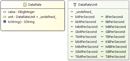
Deviations used to model constant values, histograms and statistical distributions within AMALTHEA. There is a wide variety of possible use cases, where such a distribution is needed. For example, the variation in runtime of functions can be imitated. Therefore, AMALTHEA currently supports the following statistical distributions:
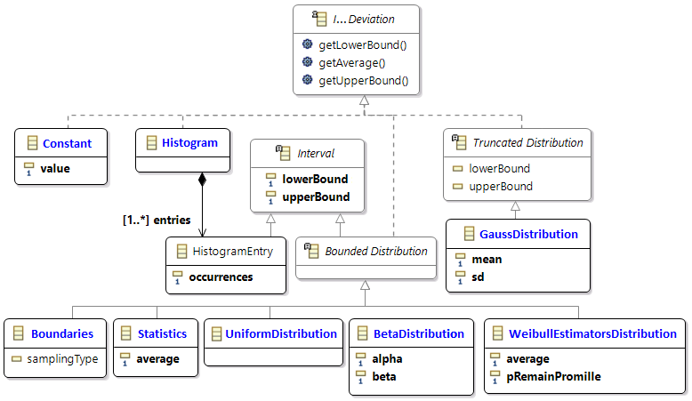
The earlier implementation used Generics to support the different use cases. To simplify the usage (via Java API and in the editor) the new implementation provides three different top level interfaces for
Time Deviation,
Discrete Value Deviation (integer values) and
Continuous Value Deviation (float values). They provide specialized methods to handle their values and a common interface to access lower bound, upper bound and average.
The following image shows the detailed hierarchy of time deviations, the other implementations are built accordingly.
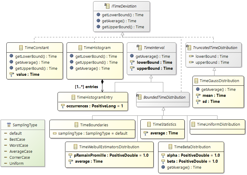
Boundaries
With the
Boundaries class it is possible to specify commonly used deviations (scenarios). On the one hand, the scenario specified by the minimum and maximum value between which the sampled values vary. On the other hand, the
Sampling Type denotes the specific scenario that is covered. These scenarios are actually defined by a Beta Distribution with preconfigured Alpha and Beta parameters. The following sampling types are available (visualized in the figures below):
- BestCase
- Defines the scenario in which most instances should have runtimes close to the specified minimum runtime, but still should consider some more time-consuming outliers up to the set maximum. Alpha = 0.2; Beta = 1.
- WorstCase
- Defines the scenario in which most instances should have runtimes close to the specified maximum runtime, but still should consider some less time-consuming outliers down to the set minimum. Alpha = 1; Beta = 0.2.
- AverageCase
- Defines the scenario in which most instances should have runtimes close to the middle between the specified minimum and maximum, but still should consider some more or less time-consuming outliers down to the set minimum or up to the set maximum respectively. Alpha = 2; Beta = 2.
- CornerCase
- Defines the scenario in which most instances should have runtimes close to the specified minimum and maximum runtime, but still should consider some other time-consuming outliers between those two. Alpha = 0.2; Beta = 0.2.
- Uniform
- Defines the scenario in which all instances should have runtimes that are uniformly distributed between the specified minimum and maximum. Alpha = 1; Beta = 1.
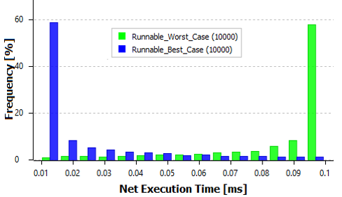
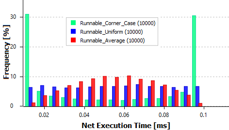
Uniform Distribution
The uniform distribution is a statistical distribution where the values between the stated lower and upper bound are equally likely to be observed.
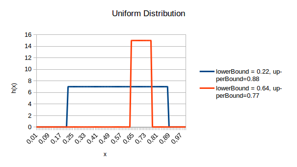
Gaussian/Normal Distribution
The Gaussian/normal distribution is a statistical distribution where the values decrease symmetrically. The maximum value and thus its location is thereby stated by the mean and the rate of decrease is defined by its standard deviation. Since the curves approach zero on either side, an additional upper and lower bound can be added to constraint the values.
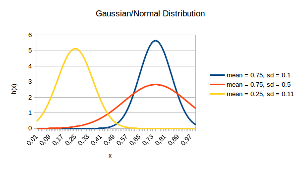
Beta Distribution
The Beta distribution is a statistical distribution whose shape is defined by alpha > 0 and beta > 0. That way, the Beta distribution can also be used to model other distributions like for example uniform, normal, or Bernoulli distribution. Since the curves can approach zero or infinity on either side, an additional upper and lower bound can be added to constraint the values.
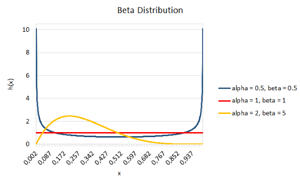
Weibull Distribution
The Weibull distribution is a statistical distribution whose shape is mathematically defined by kappa > 0 and the scale of the distribution by lambda > 0. In the model, it is parameterized using the mean value, the lower and upper bound, and the probability that a real-valued random variable of that distribution will not take a value less than or equal to a specific value. To calculate the scale and shape parameter for the Weibull distribution from the model parameters, the equation of the mean ( see
Weibull distribution – Wikipedia ) is solved for the scale parameter, first. Then, the resulting equation for lambda is plugged into the equation of the cumulative distribution function (CDF) for the Weibull distribution. Finally, the lower and upper bound allow to shift this function and the remaining unknown shape parameter in the equation is numerically approximated until the value of the parameter that constraints the distribution regarding the per mill of remaining values is reached.
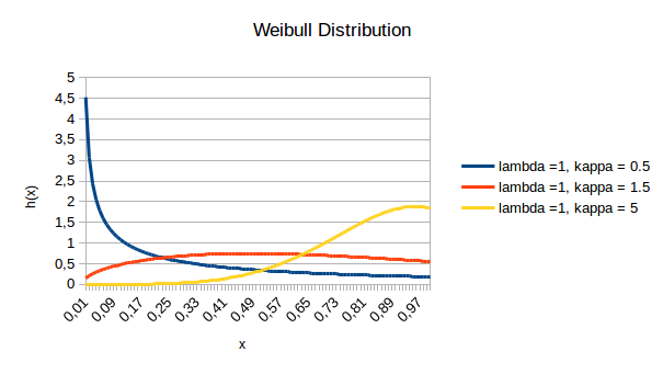
Histogram
A histogram represents a distribution containing a limited number of entries (e.g. extracted from a trace). Each entry thereby is an
Interval with the extra attribute
occurrences which holds the number instances within the interval. The intervals do not have to cover a continuous range nor do they need to have the same interval size. Histograms are useful if there is a limited number of possibilities of valuations, which covers most practical systems. See the following figure for an example of two runnables having a time histogram deviation of their execution times.
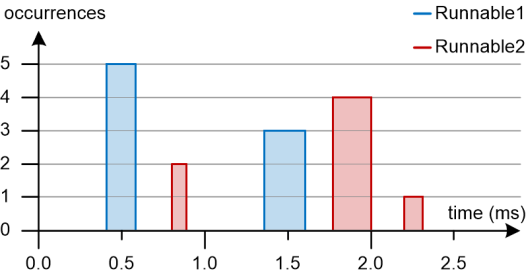
3.2.7 Statistic Elements
The contained elements are representing statistical values.
The values can be set either with a min, avg and max representation using the
MinAvgMaxStatistic element.
The other possibility is to set a single value using the
SingleValueStatistic element.
The minimum and maximum values are set as a normal
int value, the average the single value as
float.
Ticks are used to express execution times in a basic way. The number of ticks characterizes the amount of computation that is necessary to execute e.g. a
Runnable. The corresponding execution time can be easily calculated if the frequency of the executing
ProcessingUnit (PU) is known.The corresponding execution time can be easily calculated if the frequency of the executing
ProcessingUnit (PU) is knownexecution time can be easily calculated if the frequency of the executing
ProcessingUnit (PU) is known. Depending on the capabilities of a PU the time to execute such an element will differ. If necessary the fundamentally different numbers for specific types of PUs can be stored as extended values in a map.
In the next picture
Ticks are shown in more detail.
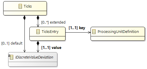
| Name |
Description |
|
default
|
The default number of ticks. This value is used if (1) the executing PU is unknown or (2) no extended entry is available for the PU. |
|
extended
|
Possibility to store a PU-specific number of ticks. |
The
Counter element describes an activation of a target element that happens only every nth time.
| Name |
Description |
|
prescaler
|
Gives the number n for the activation,
e.g. if set to 2, the target element is executed every second time. |
|
offset
|
Initial shift for the first execution of the target. |
If for example
prescaler is 5 and
offset is 2 it is executed on the 2nd, 7th, 12th, … time.
Counters are available at the following elements:
- Activity graph items:
-
ClearEvent
-
EnforcedMigration
-
InterProcessActivation
-
SchedulePoint
-
SetEvent
-
TerminateProcess
-
RunnableCall
-
WaitEvent
- Stimuli:
-
InterProcess
-
EventStimulus
Conditions are used to model the conditional execution of high level elements (Runnables, Stimuli) and also the repeated or conditional execution in a detailed activity graph (Switch, WhileLoop). The conditions have a predefined structure of top level disjunction (OR) with conjunctions (AND) or single conditions as contained elements. It is similar to the disjunctive normal form (DNF) of a logical formula.
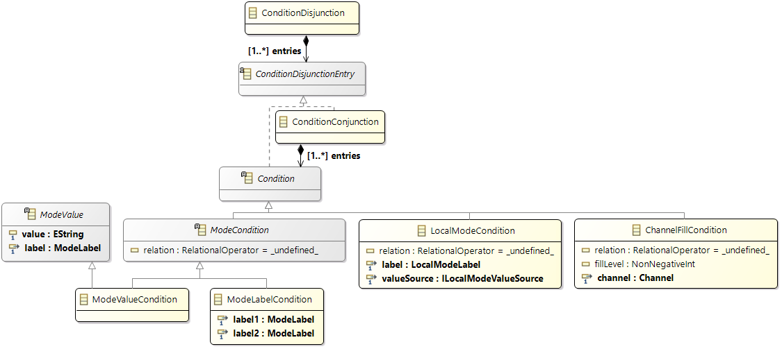
Use of common conditions:
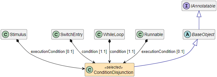
3.3 Common Elements
The
CommonElements model provides a central container for tags and classifiers. These elements are used in many sub models where references to
Tags or
Classifiers provide a mechanism to annotate objects.
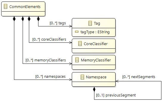
Tags are a generic possibility to annotate objects in the AMALTHEA model.
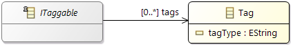
3.3.2 Classifiers
Classifiers are used to define specific features or abilities of a core or a memory. They are used in the
PropertyConstraintsModel to restrict the allocation to cores or the memory mapping.
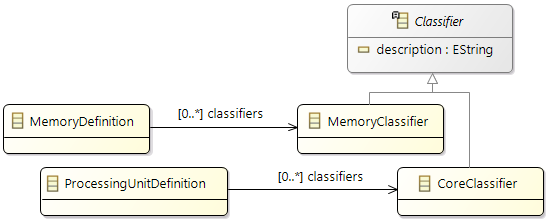
3.3.3 Namespaces
Some elements in the data model can refer to a
Namespace. A namespace provides a prefix to the name of the element.
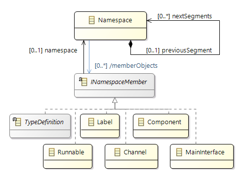
3.4 Components Model
The AMALTHEA component model is central accessible through the
ComponentsModel element.
It holds the following types:
-
Components /
Composites
-
Systems
-
Interfaces
-
Structures
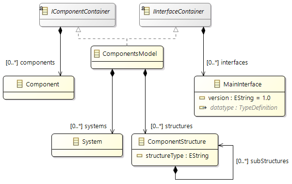
3.4.1 Component Interfaces
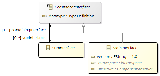
3.4.2 Architecture of Systems / Composites
The inner architecture of a System or a Composite is defined with the ISystem interface. Both elements contain component instances and connectors. The ports of the instances and the containing architecture can be identified as QualifiedPort.
3.4.3 Components Model Elements
The elements of the Components Model inherit several capabilities from common elements.
Ports, Components, Composites and ComponentInstances are referable by unique names.
A Connector also has a name but the name is optional and does not have to be unique.
Component
The 'Component' class represents a component. Components could be created directly within the 'ComponentModel' and are used as a type for a component instance.
It contains several ports of type 'Port'. A component refers the classes 'OsEvent', 'Label', 'Runnable' and 'AbstractProcess' from the software model and the class 'Semaphore' from the OS model.
System and Composite
Systems are defined as top level elements within a component model. A system contains several Component- and
Connection-instances and is used to define the architecture of a technical system.
A 'Composite' is a special component type to aggregate Component- and Connection-instances compositely.
So it could be used to create hierarchical component architectures.
System and Composite implement the interface 'ISystem'.
The following diagram shows the main elements to represent the hierarchical architecture.
In general each inner port should be connected. If a port is intentionally left unconnected it has to be added to the list of 'groundedPorts'.
ComponentInstance and Connector
The 'ComponentInstance' and the 'Connector' can be created within a 'System' or a 'Composite'. 'ComponentInstances' are used to represent instances of component- or composite-types. The 'Connector' class is used to connect the component instances to each other via their Ports. The connector contains a source and target 'QualifiedPort'.
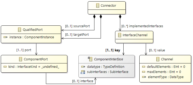
To specfiy the implementation details of a connection between ports it is possible to specify an interface/channel pair for each connector. This links additional information from the channel implementation like the access behavior to the connector. The connector can contain multiple interface/channel pairs since an interface can contain multiple sub-interfaces realized by multiple data types implemented by multiple channels.
QualifiedPort
A 'qualified' port refers a 'ComponentInstance' and a 'ComponentPort'.
If the 'instance' link is null then the QualifiedPort refers to a port of the enclosing composite.
ComponentPort
The 'ComponentPort' class contains the attribute 'kind' to set the port direction.
The attribute 'interface name' can be used to refer to an external definition, e.g. described in detail with the Franca IDL.
Structures
Structures enables structuring/ordering of components, composites and interfaces. In contrasts to namespaces the structure does not add to the qualified name but supports the design of a hierarchical structure to order the elements in a package/folder like scheme.
Diagram
The diagram of the example shows a composite 'A' that contains two component instances 'X' and 'Y' of type 'B'. The connections between the ports are named 'c1' to 'c4'. The grounded port 'in_3' of instance 'X' (intentionally left unconnected) is marked green. The second unconnected port 'in_2' of instance 'Y' is unspecified. It is marked red and has to be changed, either declared as grounded or connected to another port.
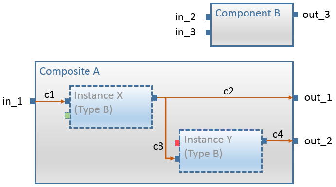
Model Editor
The same example is shown in the standard AMALTHEA editor.
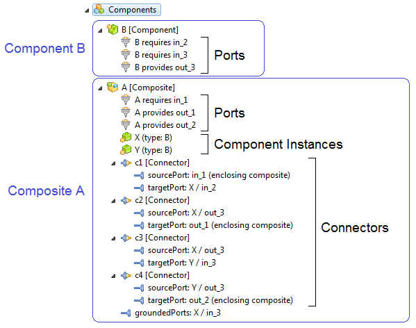
3.5 Configuration Model
The purpose of the configuration model is to provide a common mechanism for configuration purposes. The included configurations can contain elements for further processing or build steps.
The central element is the
ConfigModel class.
Currently the only configuration object is
EventConfig.
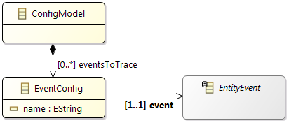
3.5.1 Event Configuration
The event configuration represents target events to trace, either in a simulation or on a target hardware platform. The
EventConfig elements are contained in the ConfigModel class as list with the name
eventsToTrace. Attributes of
EventConfig are:
-
name: (optional) name of the element
-
event: reference to an existing events in the
Events model
Sample
An example use case can be to trace all
Process activate events. To express this in the configuration, one contained element must be of type
EventConfig with the corresponding
Event pointing to an already existent element. The
Event is of type
ProcessEvent and the
ProcessEventType is set to
activate. The other attributes are left blank to not limit the configuration to one
Process with a given name for example.
The consumer of the configuration must then match and filter the relevant elements for further processing.
The following screenshot is showing this minimal configuration.
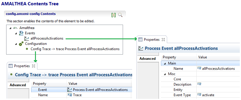
3.6 Constraints Model
The constraints model contains different kind of constraints. There are the runnable-sequencing-constraints that can be used to define a required order for the runnables of the Software Model, the affinity constraints for defining the constraints for the mapping of runnables, processes and schedulers, and the timing constraints for restricting the time span between events or the duration of event chains. Regarding to that, it is also possible to define event chains in this model.
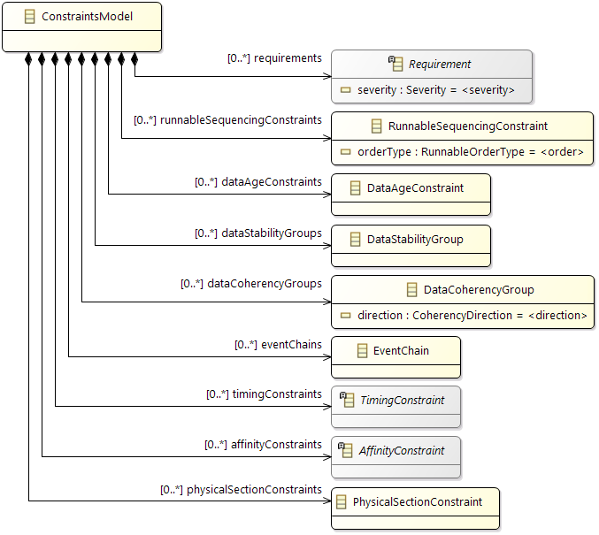
3.6.1 Requirements
The Requirements are used to specify quality requirements for the dynamic architecture.
Requirements are divided into the following types depending on the entity type for which the requirement is specified:
- Architecture Requirements for components
- Process Chain Requirements for process chains
- Process Requirements for tasks and ISRs
- Runnable Requirements for runnables
The Severity attribute is used to describe the quality impact if the requirement is not fulfilled.
The Limit defines the metric, the value, and whether the value for the metric is an upper or a lower bound.
Depending on the metric unit, the following Limits can be distinguished:
- Count Requirement Limit for metrics that count system actions
- CPU Percentage Requirement Limit for metrics that specify relative CPU characteristics
- Frequency Requirement Limit for metrics that measure the frequency of system actions
- Percentage Requirement Limit for metrics that specify relative system characteristics
- Time Requirement Limit for metrics that describe time intervals
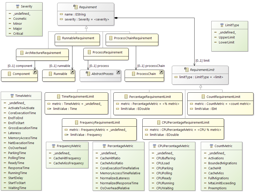
Time Metrics
Time Metrics groups all metrics that describe time intervals of an individual process instance or between two succeeding process instances and are defined here. Note that the colors of the various time slices depicted here, directly correspond to the states and colors from the BTF specification. The metrics for individual process instances include the following:
-
CoreExecutionTime
: This metric quantifies the amount of time of a process instance between its start and termination in which it is actively executed on a specific processing unit.
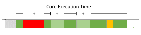
-
GrossExecutionTime
: This metric indicates the time interval between the start moment and the termination moment of a process instance.
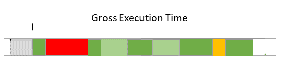
-
Lateness
: This metric indicates whether a process instance misses its deadline. It quantifies the amount of time between the termination moment of the process instance and its deadline. Thus, the resulting lateness is negative and indicates that no deadline miss occurred if the termination moment of the process instance is before the deadline and vice versa.
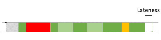
-
MemoryAccessTime
: This metric quantifies the amount of time that is required by a process for transferring data from or to the memory.
-
NetExecutionTime
: The net execution time indicates the actual execution time of a process instance, i.e., the time it is occupying a processing unit. Thus, it quantifies the time from the start moment of a process instance to its termination moment excluding the time the process instance is interfered.
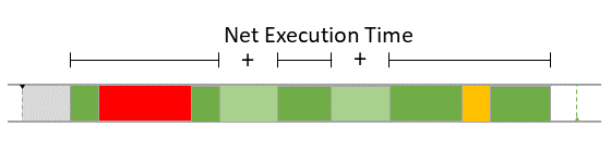
-
OsOverhead
: This metric indicates the amount of execution time that is consumed by functions that are part of the operating system.
-
ParkingTime
: This metric quantifies the amount of time that a process instance spends between its start and termination passively waiting for the access of a resource.
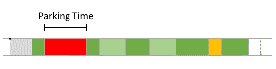
-
PollingTime
: This metric quantifies the amount of time that a process instance spends between its start and termination actively waiting for the access of a resource.
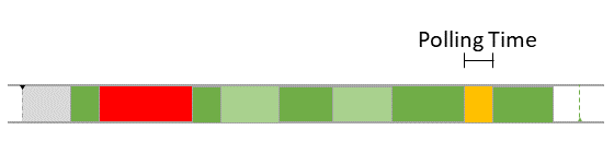
-
ReadyTime
: This metric quantifies the amount of time of a process instance between its start and termination in which it is not actively executed on any processing unit.
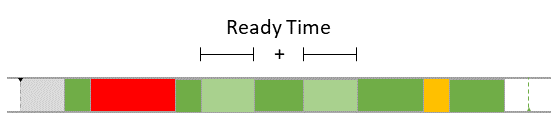
-
ResponseTime
: The response time of a task or ISR instance is defined as the time between the moment of its activation and its termination. Thus, it measures the whole life cycle of a process instance.
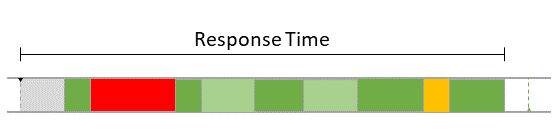
-
RunningTime
: This metric quantifies the amount of time of a process instance between its start and termination in which it is actively executed on any processing unit.
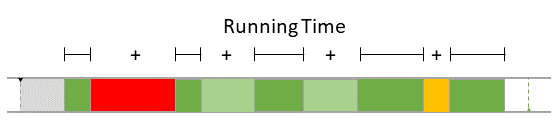
-
StartDelay
: This metric quantifies the delay of the start time of a process instance which is defined as the time interval between the activation moment of this process instance and its start moment.
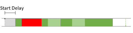
-
WaitingTime
: This metric quantifies the amount of time that a process instance spends between its start and termination passively waiting for an OS event.
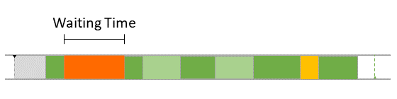
Inter Process Instance Metrics
Inter Process Instance Metrics include the following:
-
ActivateToActivate
: This metric indicates the distance between two successive activations of a task or isr. The
ActivateToActivate metric of process instance n quantifies the time between the activation moment of process instance n and that of instance n+1.
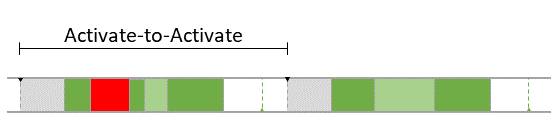
-
EndToEnd
: This metric indicates the time interval between two successive ends of a process. The
EndToEnd metric of process instance n quantifies the time between the termination moment of process instance n and that of instance n+1.

-
EndToStart
: This metric indicates the time interval between two successive process instances. The
EndToStart metric of process instance n quantifies the time between the termination moment of process instance n and the start moment of instance n+1.
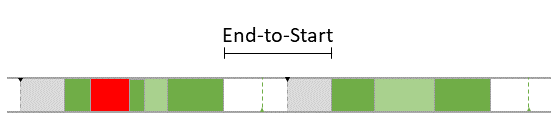
-
StartToStart
: This metric indicates the time interval between two successive starts of a process. The
StartToStart metric of process instance n quantifies the time between the start moment of process instance n and that of instance n+1.
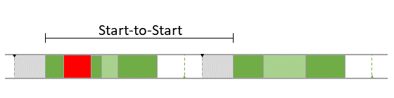
Count Metrics
Count Metrics groups all metrics that describe absolutely how often system characteristics occur and are defined as follows:
-
Activations
: This metric quantifies the number of times a process is activated.
-
BoundedMigrations
: This metric quantifies the number of times a process instance starts executing on a processing unit that is different to the processing unit on which the previous process instance terminated.
-
CacheHit
: This metric quantifies the amount of times that data requested by a process is found in the cache memory.
-
CacheMiss
: This metric quantifies the amount of times that data requested by a process is not stored in the cache memory and has to be fetched from somewhere else.
-
FullMigrations
: This metric quantifies the number of times a process instance migrates from one processing unit to another triggered by a schedule point.
-
MtaLimitExceeding
: This metric quantifies the number of times a process is not activated during runtime because this would violate the maximum number of concurrently activated processes (MTA).
-
Preemptions
: This metric quantifies the number of times a process is preempted by another task or ISR.
Frequency Metrics
Frequency Metrics groups all metrics that describe the rate in which system characteristics occur and are defined as follows:
-
CacheHitFrequency
: This metric quantifies how often per unit of time data requested by a process is found in the cache memory.
-
CacheMissFrequency
: This metric quantifies how often per unit of time data requested by a process is not found in the cache memory.
CPU Percentage Metrics
CPU Percentage Metrics groups all metrics that describe a ratio between the amount of time a processing unit is in a certain state for a specific process and the maximum capacity of the considered processing unit and are defined as follows:
-
CPUBuffering
: This metric quantifies the ratio between the amount of time a processing unit is in the state buffering for a specific process and the maximum capacity of the considered processing unit.
-
CPULoad
: This metric quantifies the ratio of the load of a processing unit caused by a process and the maximum capacity of the considered processing unit.
-
CPUParking
: This metric quantifies the ratio between the amount of time a processing unit is in the state parking for a specific process and the maximum capacity of the considered processing unit.
-
CPUPolling
: This metric quantifies the ratio between the amount of time a processing unit is in the state polling for a specific process and the maximum capacity of the considered processing unit.
-
CPUReady
: This metric quantifies the ratio between the amount of time a processing unit is in the state ready for a specific process and the maximum capacity of the considered processing unit.
-
CPURunning
: This metric quantifies the ratio between the amount of time a processing unit is in the state running for a specific process and the maximum capacity of the considered processing unit.
-
CPUWaiting
: This metric quantifies the ratio between the amount of time a processing unit is in the state waiting for a specific process and the maximum capacity of the considered processing unit.
Percentage Metrics
Percentage Metrics groups all metrics that describe a relationship between two system characteristics and are defined as follows:
-
CacheHitRatio
: This metric quantifies how often data requested by a process is found in the cache memory in comparison to how often it is not found.
-
CacheMissRatio
: This metric quantifies how often data requested by a process is not found in the cache memory in comparison to how often it is found.
-
NormalizedLateness
: This metric quantifies the lateness of a process instance in comparison to the process's maximum response time which is defined by its deadline.
-
NormalizedResponseTime
: This metric quantifies the response time of a process instance in comparison to the process's maximum response time which is defined by its deadline.
-
OsOverheadRelative
: This metric quantifies the amount of execution time that is consumed by functions that are part of the operating system in comparison to net execution time of the process in whose context the functions are called.
An example for a requirement is the deadline for a task. The deadline is specified by an upper limit for the response time of the respective task.
3.6.2 Runnable Sequencing Constraints
These constraints can be used to define execution orders of runnables or, in other words, the dependencies between runnables. These dependencies can result from data exchange or any functional dependency that is not necessarily visible by other model parameters.
The following requirements can be specified with this constraint:
- Execution sequence of runnables A ->B, meaning A has to be finished before B starts
- Scope on certain process/processes, when a runnable is executed multiple times in different process contexts
- Succession of runnables within a process (strict, loose)
- Position of sequence within a process (start, end, any position)
A
RunnableSequencingConstraint contains a list of
ProcessRunnableGroup elements and an enumeration
RunnableOrderType describing the basic rule for the sequencing. In general, a runnable sequencing constraint is independent of the processes that execute the runnables. Via the attribute "processScope" it is possible to define that a sequencing constraint is only valid for runnables within just one process or a set of processes.
The
ProcessRunnableGroups contain references to runnables that should be sequenced. The sequence is defined by the order of the runnable groups within the sequencing constraint. The order of the runnable references within a group is undefined.
To sequence two runnables it is consequently necessary to create a
RunnableSequencingConstraint with two
ProcessRunnableGroups, each referencing one of the runnables.
To describe that a set of runnables have to be executed before or after another runnable or set of runnables, it is possible to put more than one runnable reference in a group. As already mentioned, the order of the referenced runnables within a
ProcessRunnableGroup is unimportant.
The following picture visualises a
RunnableSequencingConstraint and multiple possible runtime situations. The constraint has two runnable groups, each depicted by an ellipsis. In this example, there is just one runnable in each group. The runnables in the groups must be executed in the order of the group ("R1" before "R2"). There is no restriction in which process context the runnables are executed. It is important that the order is correct and that the runnable of one group terminates before the runnable of the next group starts. The exemplary runtime situations shown in the lower part of the figure visualise situations that satisfy this constraint (blue) and those who violate the constraint (red).
The
RunnableSequencingConstraint in the next figure has two processes set as a scope in its second group. That means that the runnable "R3" is allowed to be executed on the processes "P1" or "P3" (blue). But it is only expected to be executed one time in between (red)!
Each
RunnableSequencingConstraint has a
RunnableOrderType. It provides the following sequencing modes:
- successor
- immediateSuccessorAnySequence
- immediateSuccessorEndSequence
- immediateSuccessorStartSequence
The meaning of the mode "successor" is that the runnable groups of a sequencing constraint do not have to follow each other directly, i.e., runnables that are not part of the constraint can be executed in between.
In contrast to this, the modes starting with "immediateSuccessor" express that the runnables referenced by the runnable groups must execute in direct order, so without any runnable in between. With "StartSequence", "AnySequence" and "EndSequence" it is further constrained that the runnables of the constraint have to be executed at the beginning, at the end or at any position in a process.
Assuming that all runnables are executed on the same process, the mode "immediateSuccessorStartSequence" means that all runnables of the constraint have to be executed in the correct order at the beginning of the process.
The mode "immediateSuccessorEndSequence" is like "immediateSuccessorStartSequence", but here the runnable sequence must be executed at the end of the process.
3.6.3 Data Age Constraints
Data Age constraints are used to define when the information in a label becomes valid or invalid after its last update. Therefore a runnable and a label has to be set. The information update occurs when the runnable performs a write access on the label. It is possible to define the minimum time after the information of a label update becomes valid. This means that the information shall not be used for further calculations before this time is over. The maximum time on the other hand defines the time after the label update when the information becomes invalid. Beside of time it is possible to define a minimum and maximum cycle. The cycle is related to the activation of the process that executes the runnable.
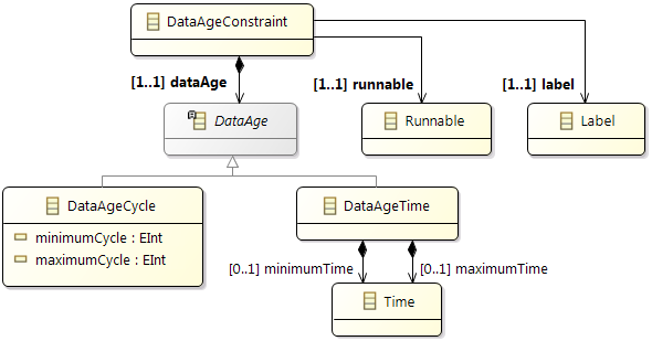
- DataAgeTime: The
Time object in the role of
minimumTime must not contain a negative value!
- DataAgeTime: The
Time object in the role of
maximumTime must not contain a negative value!
3.6.4 Data Coherency Groups
A
DataCoherencyGroup is used to define data coherency requirements for a group of labels.
The Direction hereby is used to specify if the labels have to be read or written coherently. Moreover, the scope attribute defines the context of the coherent read or write requirement. Possible scopes are components, processes, and runnables.
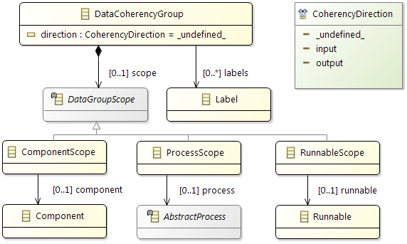
3.6.5 Data Stability Groups
A
DataStabilityGroup is used to define that the values of labels have to be kept stable within a given execution context.
Currently, the following execution contexts are covered by the scope:
- Component
- Process
- Runnable
This means that it has to be guaranteed that the values of labels are identical either within the runnable, the process, or the component in which the denoted labels are accessed.
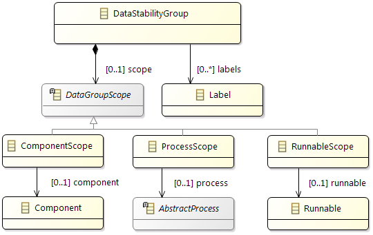
3.6.6 Event Chains
The concept for event chains is based on the Timing Augmented Description Language.
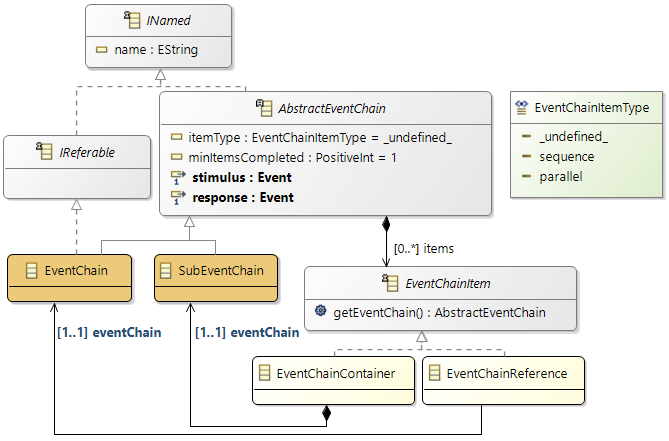
The
EventChain consists of
EventChainItems. These items are classified in two types:
- EventChainReferences -> EventChain: Used to refer to already defined EvenChains.
- EventChainContainers -> SubEventChain: Inner anonymous EventChains, which are only available in the context of the current EventChain.
An Event Chain object references always two events, a stimulus event and a response event. To define a simple event chain that just contains two events, one event chain object is enough. In this case it would just be a chain that with its stimulus as first event and the response as second event.
If more events are required it is necessary to add sub event chains. The stimulus is always the first event of an event chain, the response is always the last event. The events that are defined in the sub event chains are the events in between.
When adding
EventChainItems there are two properties that decide on the semantics of the SubEventChains:
| Name |
Description |
|
EventChainItemType
|
This property defines how to interpret the subEventChain. There exist two possibilities:
sequence and
parallel. Sequence means that all the subEventChains are evaluated in the defined order of the list. Parallel path can be alterantive paths or joins.
|
|
minItemsCompleted
|
Defines how the parallel execution is interpetated. The designer specifies how many elements of the subEventChains must be completed to go to the next step.
1 represents alternative paths of the EventChain. If the number equals the number of elements in the
EventChainItems list all paths must be triggered to continue the event-chain tracking and represents a complete join of all subEventChains
|
Simple structural example for sequence
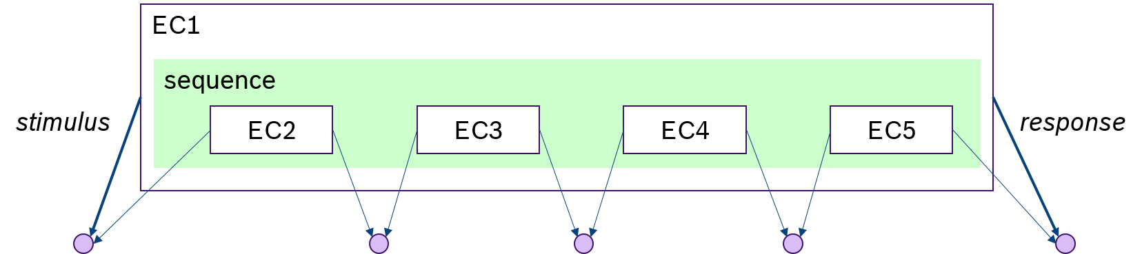
Simple structural example for parallel paths
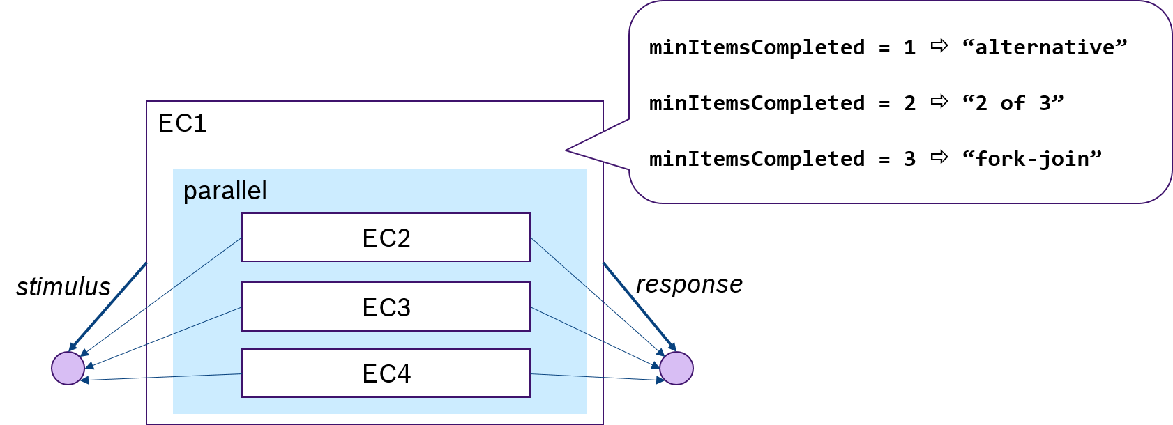
Structural example how to combine both
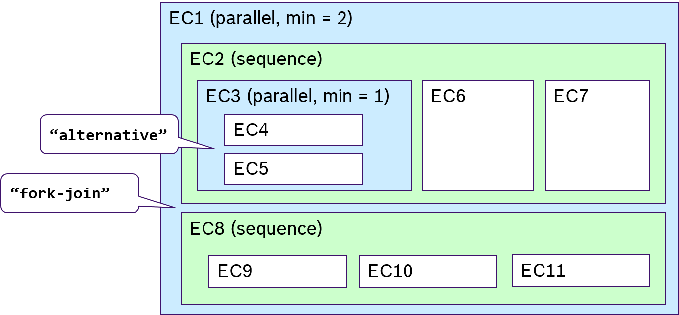
The picture below shows a simple example for an event chain of four events in a row.
The top level chain defines the first event (E1) and the last event (E4).
It contains a number of event chains. They describe the way from E1 to E4.
These sub event chains are added as
sequence to the parent.
For this some rules has to be considered:
The stimulus of the first child event chain has to be the same as the stimulus of the parent (red in picture).
The stimulus of other child event chains have to be equal to the response of the previous chain (blue in picture).
The response of the last child event chain has to be the same as the response of the parent (green in picture).
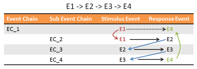
As a stimulus or response event it is either possible to use an Entity Event or an Event Set.
An Entity Event is a single event regarding to an entity like a task or a runnable. So it can be e.g. the start of a runnable.
If a set of events is used, then all events of this group must occur fulfill the event chain. The order in which the events occur is not important.
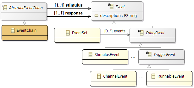
3.6.7 Timing Constraints
Synchronization Constraints
An
EventSynchronizationConstraint describes how tightly the occurrences of a group of events follow each other.
There must exist a sequence of time windows of width tolerance, such that every occurrence of every event in events belongs to at least one window, and every window is populated by at least one occurrence of every event.
The parameter
multipleOccurrencesAllowed defines, whether for the constraint all occurrences have to be considered or just the subsequent ones.
An
EventChainSynchronizationConstraint describes how tightly the occurrences of an event chain follow the occurrences of a different event chain.
The
SynchronizationType defines which parts of the event chains have to be in sync, stimulus or response, and the width of a time window sets the allowed tolerance.
The parameter
multipleOccurrencesAllowed defines, whether for the constraint all occurrences have to be considered or just the subsequent ones.
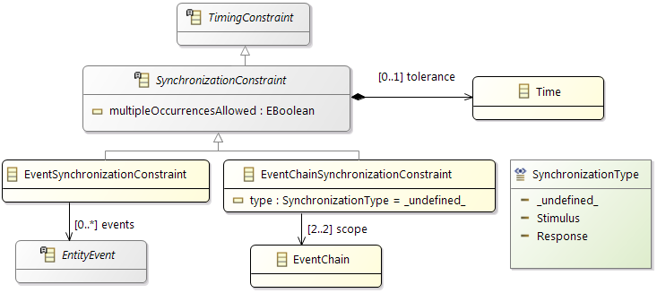
-
SynchronizationConstraint: The
Time object in the role of
tolerance must not contain a negative value!
Repetition Constraint
A
RepetitionConstraint describes the distribution of the occurrences of a single event, including jitter.
Every sequence of span occurrences of event must have a length of at least lower and at most upper time units.
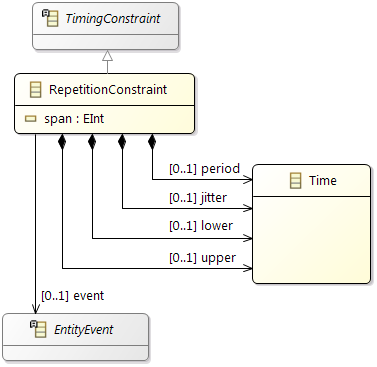
-
RepetitionConstraint: The
Time object in the role of
lower must not contain a negative value!
-
RepetitionConstraint: The
Time object in the role of
upper must not contain a negative value!
-
RepetitionConstraint: The
Time object in the role of
period must not contain a negative value!
-
RepetitionConstraint: The
Time object in the role of
jitter must not contain a negative value!
Delay Constraint
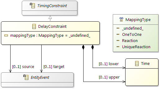
-
DelayConstraint: The
Time object in the role of
lower must not contain a negative value!
-
DelayConstraint: The
Time object in the role of
upper must not contain a negative value!
A Delay Constraint imposes limits between the occurrences of an event called source and an event called target.
Every instance of source must be matched by an instance of target within a time window starting at lower and ending at upper time units relative to the source occurrence.
A
MappingType defines whether there is a strong (
OneToOne ), neutral (
Reaction ), or weak (
UniqueReaction ) delay relation between the events:
-
OneToOne
: According to page 18f of
TIMMO-2-USE Deliverable D11 'Language Syntax, Semantics, Metamodel V2', a constraint with this mapping type is satisfied if and only if
source and
target have the same number of occurrences and for each index
i, if there is an
i-th occurrence of source at time
x there is also an
i-th occurrence of
target at time
y such that
lower ≤
y -
x ≤
upper.
This means that the source event and the target event have the same number of occurrences and no stray target occurrences are accepted.
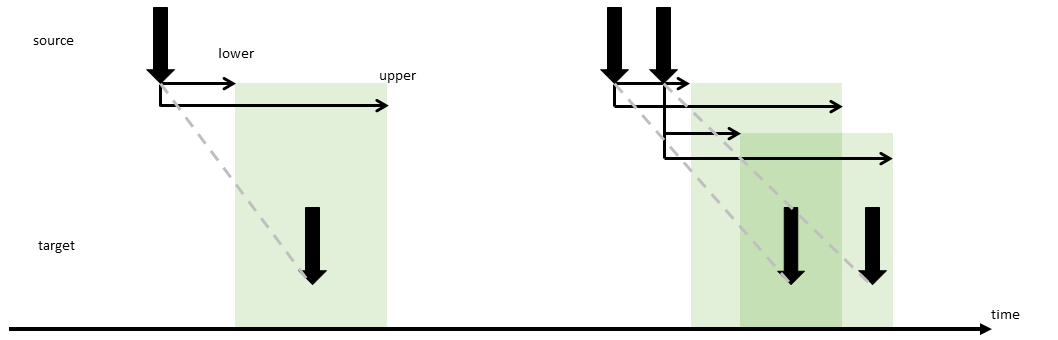
-
Reaction
: According to page 17f of
TIMMO-2-USE Deliverable D11 'Language Syntax, Semantics, Metamodel V2', a constraint with this mapping type is satisfied if and only if for each occurrence
x of
source, there is an occurrence
y of
target such that
lower ≤
y -
x ≤
upper.
This means that multiple source event occurrences may be mapped to the same target event and stray target event occurrences are ignored.
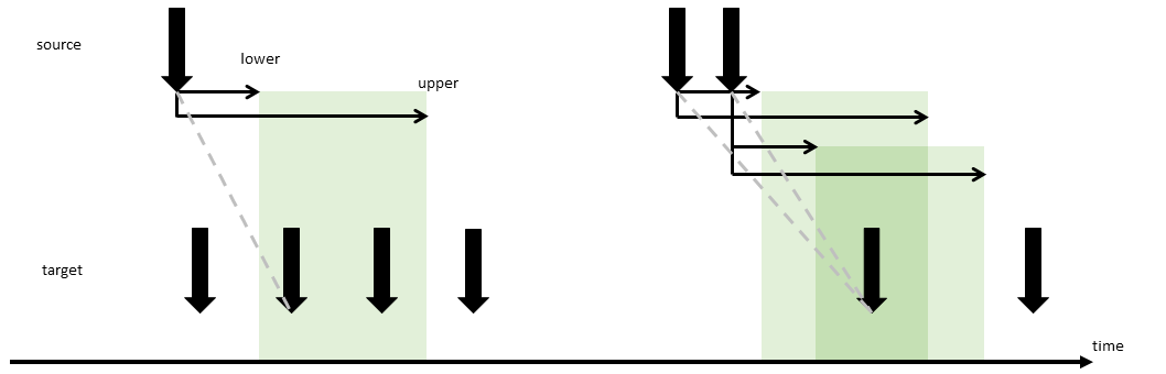
-
UniqueReaction
: This mapping type is a mixture of the previous types by specifying that for every occurrence of the source event exactly one target event must occur within the defined time span. Thus, target events may not be shared between source events and stray target events violate the requirement. In contrast to the
OneToOne mapping case, the source event is not mapped to the first source event but is dropped as a violation, if a target event is missed.
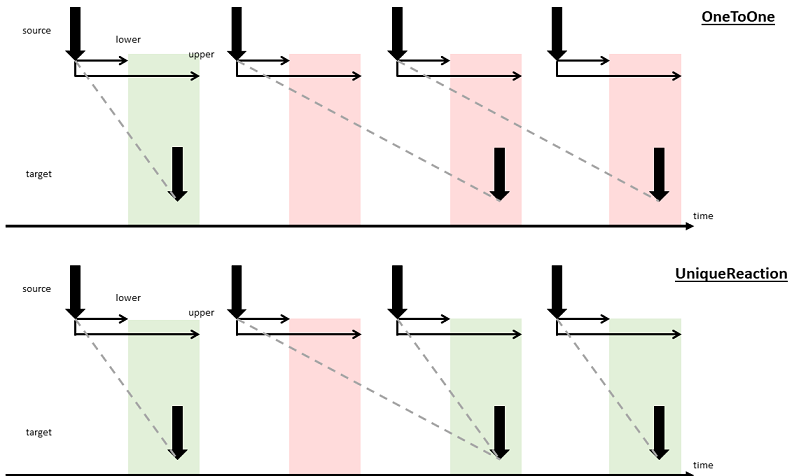
Event Chain Latency Constraint
An
EventChainLatencyConstraint defines how long before each response a corresponding stimulus must have occurred (
Age ), or how long after a stimulus a corresponding response must occur (
Reaction ).
It always refers to an EventChain.
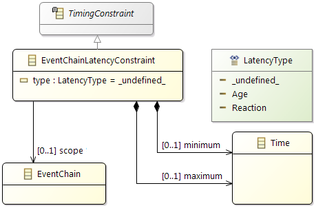
-
EventChainLatencyConstraint: The
Time object in the role of
minimum must not contain a negative value!
-
EventChainLatencyConstraint: The
Time object in the role of
maximum must not contain a negative value!
3.6.8 Affinity Constraints
Affinity constraints are used to define the mapping of executable objects to each other.
The objects that can be mapped are:
- Runnables
- Processes (Task or ISR)
- Labels
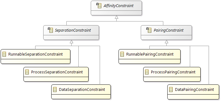
An affinity constraint can either be a pairing or a separation constraint. A pairing constraint contains one amount of objects and a target. The pairing constraints say "All these objects must run together on this target". A separation constraint contains two groups of objects and a target. It says "This group of objects is not allowed to be mapped with the other group of objects on the specific target". So the separation constraint can be used to forbid a combination of objects on a target. It can also be used to say "These objects are not allowed to be mapped on this target". In this case only one group of the separation constraint is used.
Each affinity constraint has one or more targets. The type of the target depends on the type that should be mapped.
Data Affinity Constraints
A
DataConstraint is used to define the mapping of label objects to memory units.
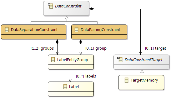
Process Affinity Constraints
A
ProcessConstraint is used to define the mapping of process (Task or ISR) objects to processing cores or scheduling units.
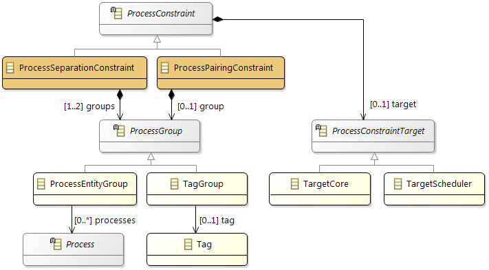
Runnable Affinity Constraints
A
RunnableConstraint is used to define the mapping of runnable objects to processing cores or scheduling units.
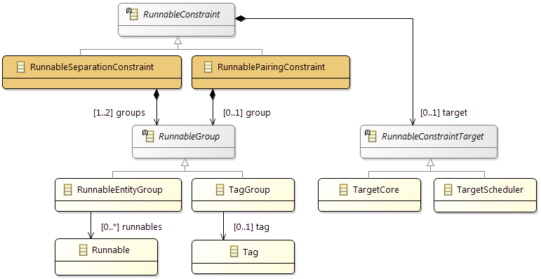
3.6.9 Physical Section Constraints
A
PhysicalSectionConstraint is used to to define the mapping of Section objects to Memories. This mapping of Section object to Memory objects specifies that corresponding
PhysicalSectionMapping associated to this
Section element can be allocated only in the mapped Memories.
Example: PhysicalSectionConstraint with the below properties has the following semantic:
	name: Ram1_Ram2_PhysicalSectionConstraint
	Memories : RAM1, RAM2
	Section : .abc.reini
Semantic: PhysicalSectionMapping for .abc.reini section can only be allocated either in RAM1 or RAM2 or in both. But not in other Memories.
3.7 Event Model
The event model provides the classes to describe the BTF-Events that can be used for the tracing configuration, for the modeling of event chains and for some timing constraints.
The top level structure is the following:

There are different event classes for the different entity types that can be traced:
| Entity |
Event Class |
| Process (Task, ISR) |
ProcessEvent |
| ProcessChain |
ProcessChainEvent |
| Stimulus |
StimulusEvent |
| Runnable |
RunnableEvent |
| Label |
LabelEvent |
| ModeLabel |
ModeLabelEvent |
| Channel |
ChannelEvent |
| Semaphore |
SemaphoreEvent |
| Component |
ComponentEvent |
3.7.1 Entity Events

3.7.2 Trigger Events

3.7.3 Process Events
In a running system, each entity can have different states. An event trace consists of the events that are visualizing the state-transitions of the traced entities. To define such an event in the model, each kind of event class contains an event-type-enumeration that provides the event-types for the state-transitions of its entity. The following picture shows the possible states of a process:

So for example the event-type-enumeration for a process event contains the events
activate,
start,
resume, ...
A description of the individual events can be found in the following table:
| Event Class |
Event Type |
Description |
| ProcessEvent |
activate |
The process instance is activated by a stimulus. |
| start |
The process instance is allocated to the core and starts execution for the first time. |
| resume |
The preempted process instance continues execution on the same or other core. |
| preempt |
The executing process instance is stopped by the scheduler, e.g. because of a higher priority process which is activated. |
| poll |
The process instance has requested a resource by polling (active waiting) which is not available. |
| run |
The process instance resumes execution after polling (i.e. active waiting) for a resource. |
| wait |
The process has requested a non-set OS EVENT (see OSEK 2.2.3 Extended Task Model, WAIT_Event()). |
| poll_parking |
The parking process instance is allocated to the core and again polls (i.e. actively waits) for a resource. |
| park |
The active waiting process instance is preemptedby another process. |
| release_parking |
The resource which is requested by a parking process instance becomes available, but the parking process stays preempted and changes to READY state. |
| release |
The OS EVENT which was requested by a process is set (see OSEK 2.2.3 Extended Task Model, SET_Event()) and the process is ready to proceed execution. |
| terminate |
The process instance has finished execution. |
| RunnableEvent |
start |
The runnable instance is allocated to the core and starts execution for the first time. |
| suspend |
The executing runnable instance is stopped, because the calling process is suspended. |
| resume |
The suspended runnable instance continues execution on the same or another core. |
| terminate |
The runnable instance has finished execution. |
| ComponentEvent |
start |
The execution of the component started, i.e. the first runnable in the list of runnables of the component instance is started. |
| end |
The execution of the component completed, i.e. all runnables in the list of runnables of the component instance were executed at least once. |
| ChannelEvent |
send |
A process or runnable has just sent data via the channel. |
| receive |
A process or runnable has just received data via the channel |
| LabelEvent |
read |
The read event indicates that a label is read by a process or runnable. |
| write |
The write event indicates that a label is written by a process or runnable. |
| ModeLabelEvent |
read |
The read event indicates that a mode label is read. |
| write |
The write event indicates that a mode label is written. |
| increment |
The increment event indicates that a mode label is written and the new value is greater than the old value. |
| decrement |
The decrement event indicates that a mode label is written and the new value is less than the old value. |
| SemaphoreEvent |
lock |
The semaphore has been requested by a runnable or process for a specific processing unit and reached the maximum number (usually 1) of assigned users. |
| unlock |
The semaphore has been released by a process or runnable for a specific processing unit and can now be assigned to an other user. |
If it is required to define an event like "start-event of
some process" then it is enough to create a object of type
ProcessEvent and set the event-type
start.
It is also possible to restrict the definition of an event to a special entity. So it can be defined like "start-event of task T_1". Therefore it is possible to reference a process from
ProcessEvent. In general, each event class can reference an entity of the corresponding type. In addition to that, each event class provides individual restrictions. So it is possible for
ProcessEvent that the event is not only restricted to a special process, it can be also restricted to a core. So that would be like "start-event of task T_1 on core C_2". Another example is the class
RunnableEvent, it allows to restrict the event to a runnable, the process that executes the runnable and the core that executes the process.
3.8 Hardware Model
The AMALTHEA hardware model is used to describe hardware systems which usually consist of several hierarchical elements which contain processing units, memories, connections etc. It is accessible through the
HWModel element and contains following top level elements:
- Definitions
- Domains
- Features
- Structures
3.8.1 Class Diagrams
Hardware model elements
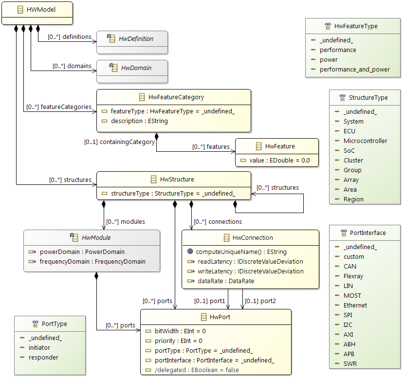
Hardware definitions and features
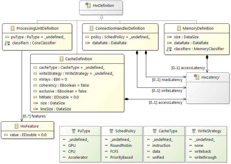
Hardware modules and access elements
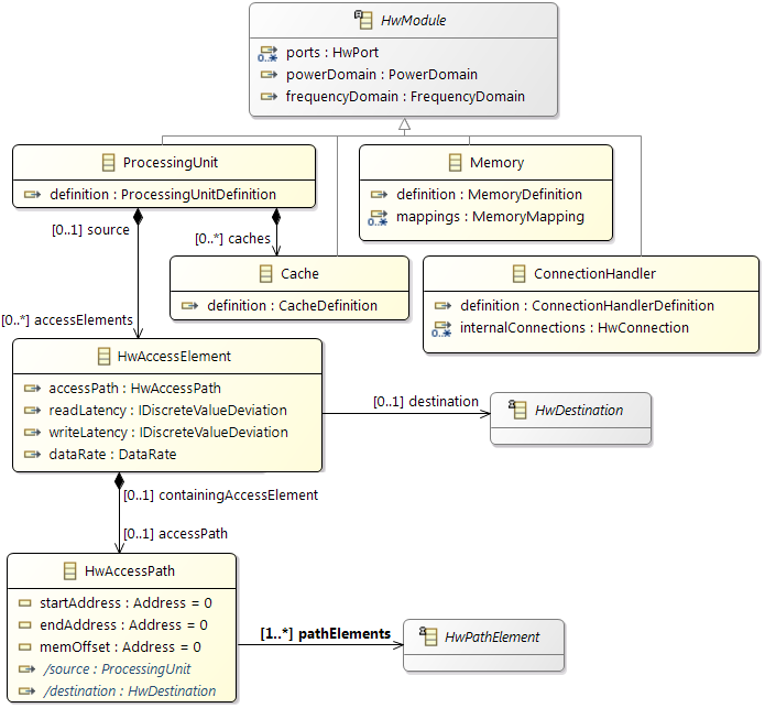
Hardware paths and destinations
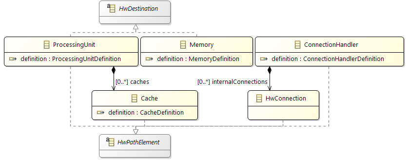
3.8.2 Element description
The following tables describe the different model elements and their attributes in detail. For several elements short examples are attached.
HwModel
The
HwModel class is the root element of the hardware model. It always contains one or multiple
HwStructures, PowerDomains and
FrequencyDomains and optionally different
HWFeaturesCategories for the
HwModule definitions.
| Attribute |
Type |
Value |
Mul. |
Description |
| Name |
String |
String |
1 |
Name of the hardware model |
| Definitions |
Containment |
HwDefinition |
* |
Definitions of ProcessingUnits, Memories, Caches and ConnectionHandlers |
| Domains |
Containment |
HwDomain |
* |
Frequency- and PowerDomains |
| FeatureCategories |
Containment |
HwFeatureCategory |
* |
FeatureCategory for the HwModel including HwFeatures |
| Structures |
Containment |
HwStructure |
* |
Hierarchical structure of the hardware model |
HwDefinition
Additional information about the definition concept in general can be found in the User Guide (see General Hardware Model Overview).
ProcessingUnitDefinition
For specifying a compute resource a
ProcessingUnitDefinition is created, which is afterwards referenced by the number of
ProcessingUnit instances of this kind. A
ProcessingUnitDefinition can reference multiple
HwFeatures to express different costs for different operations but only one
HwFeature per
HwFeatureCategory.
| Attribute |
Type |
Value |
Mul. |
Description |
| Name |
String |
String |
1 |
Name of the processing unit definition |
| PuType |
Enum |
PuType |
1 |
Type of the processing unit e.g. (Core, GPU, etc.) |
| Features |
Reference |
HwFeature |
* |
Hardware features of the definition |
MemoryDefinition
For specifying a memory, a
MemoryDefinition is created, which is afterwards referenced by the number of
Memory instances of this kind.
| Attribute |
Type |
Value |
Mul. |
Description |
| Name |
String |
String |
1 |
Name of the memory definition |
| AccessLatency |
Containment |
HwLatency |
1 |
Constant or distribution of access latency in cycles |
| DataRate |
Containment |
DataRate |
1 |
Max. data rate for the memory |
| Size |
Containment |
Size |
1 |
Size of the memory |
| MemoryType |
Enum |
MemoryType |
1 |
type of the memory (e.g. DRAM, Flash, SRAM, PCM) |
CacheDefinition
For specifying a cache, a
CacheDefinition is created, which is afterwards referenced by the number of
Cache instances of this kind.
| Attribute |
Type |
Value |
Mul. |
Description |
| Name |
String |
String |
1 |
Name of the memory definition |
| AccessLatency |
Containment |
HwLatency |
1 |
Constant or distribution of access latency in cycles |
| Size |
Containment |
Size |
1 |
Size of the memory |
| CacheType |
Enum |
CacheType |
1 |
Cache type (e.g. data, instruction) |
| WriteStrategy |
Enum |
WriteStrategy |
1 |
Cache write strategy (e.g. write-back) |
| Coherency |
Bool |
Bool |
1 |
Cache coherency (default = false) |
| Exclusive |
Bool |
Bool |
1 |
Exclusive cache (default = false) |
| Line Size |
Int |
Int |
1 |
Line size in bits |
| Hit Rate |
Double |
Double |
1 |
Percentage hit rate of the cache(default = 0.0) |
| NWays |
Int |
Int |
1 |
N ways associative (default = 0) |
ConnectionHandlerDefinition
For specifying a bus or Interconnect etc., a
ConnectionHandlerDefinition is created, which is afterwards referenced by the number of
ConnectionHandler instances of this kind.
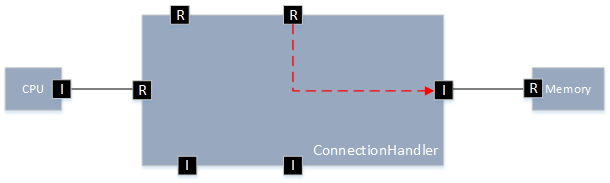
The figures shows an example of the attribute
MaxConcurrentTransfers with the default value 1. This means that all
ConnectionHandlers which are referencing this
ConnectionHandlerDefinition can only handle 1 active transfer request at a time. All other requests have to wait until the current transfers has finished.
The next figure shows an example with a number of
MaxConcurrentTransfers of 3. In this case the
ConnectionHandler can handle up to 3 concurrent requests.
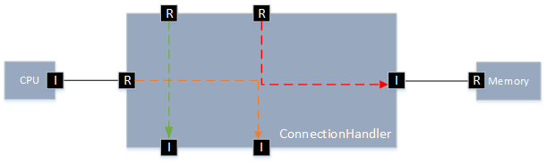
The value for
MaxConcurrentTransfers has to be smaller or equal then the min(initiator ports, responder ports).
The values for
DataRate,
ReadLatency, and WriteLatency are default values for all
ConnectionHandlers of this kind. For a specific
InternalConnection in a
ConnectionHandler instance other values can be assigned.
| Attribute |
Type |
Value |
Mul. |
Description |
| Name |
String |
String |
1 |
Name of the memory definition |
| SchedPolicy |
Enum |
SchedPolicy |
1 |
Enumeration of different scheduling policies |
| ReadLatency |
Containment |
HwLatency |
1 |
Constant or distribution in cycles for a read access |
| WriteLatency |
Containment |
HwLatency |
1 |
Constant or distribution in cycles for a write access |
| DataRate |
Containment |
DataRate |
1 |
Max. data rate of the connection (value and unit) |
| MaxBurstSize |
Int |
Int |
1 |
Maximum burst size of a ConnectionHandler (default = 1) |
| MaxConcurrentTransfers |
Int |
Int |
1 |
Number of concurrent transfers from different initiator to responder ports (default = 1) |
HwStructure
A
HwStructure is a hierarchical element which can contain all kind of
HwModules,
HwConnections and other
HwStructures. Different
HwStructures can be connected via one or more
HwPorts with other structures or modules of a top level
HwStructures. By combining different
HwStructures any kind of hierarchical system can be expressed. By setting the structure type attribute (e.g. Cluster, ECU) the structural level in the hardware is directly expressible.
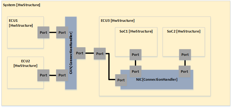
The figure shows an example for creating a hierarchy within an E/E-architecture. The
HwStructure System (which is called "System") is created as top level structure within the HwModel. It contains three other structures which represents different ECUs. The structures are connected via
HwPorts,
HwConnections and a
ConnectionHandler. Usually structures in the model can be viewed as black boxes which can be connected via
HwPorts.
ECU3 allows a look inside, where additional structures for two SoCs are visible.
| Attribute |
Type |
Value |
Mul. |
Description |
| Name |
String |
String |
1 |
Name of the hardware structure |
| StructureType |
Enum |
StructureType |
1 |
Defines the type of the structure (e.g. ECU) |
| Modules |
Containment |
HwModule |
* |
Modules of the structure (e.g. Memory) |
| Ports |
Containment |
HwPort |
* |
Ports to connect the structure (always delegated Ports) |
| Structures |
Containment |
HwStructure |
* |
Hardware structure to build hierarchical designs |
| Connections |
Containment |
HwConnection |
* |
Connections within a structure |
HwDomain
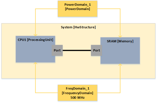
The figure shows an example for
HwDomain (
FrequencyDomain and a
PowerDomain). They are always created at the top level in the root element
HwModel. Every basic component is able to reference a
FrequencyDomain and a
PowerDomain.
(Note: The link between domains and modules are only references, there are no visible connections inside the model)
FrequencyDomain
A
FrequencyDomain is inherited from
HwDomain. This element describes a frequency domain which can be referenced by all elements of the type
HwModule to define the default frequency value for operation. In future the
FrequencyDomain should also contain possibleValues which should specify the different frequencies for different operation modes.
| Attribute |
Type |
Value |
Mul. |
Description |
| Name |
String |
String |
1 |
Name of the frequency domain |
| DefaultValue |
Containment |
Frequency |
1 |
Default frequency value |
| Clock Gating |
Boolean |
Boolean |
1 |
Possibility to power down the domain (default = false) |
PowerDomain
A
PowerDomain is inherited from
HwDomain. This element describes a power domain which can be referenced by all elements of the type
HwModule, to define the default voltage value for operation. In future the
PowerDomain should also contain possibleValues which should specify the different voltages for different operation modes.
| Attribute |
Type |
Value |
Mul. |
Description |
| Name |
String |
String |
1 |
Name of the power domain |
| DefaultValue |
Containment |
Voltage |
1 |
Default voltage value |
| PowerGating |
Boolean |
Boolean |
1 |
Possibility to power down the domain (default = false) |
HwFeature
A
HwFeature is an abstract element to represent any kind of special functionality of a
ProcessingUnitDefinition.
HwFeatures could be reused several times by different definitions and organized within
HwFeatureCategories. Currently this
HwFeatureCategories are directly referenced out of the Software Model in future the cost function (
Recipes) of an algorithm will be placed in an additional intermediate layer.
More information can be found in (see Hardware Concepts).
NOTE: The concepts "Recipe" and "Hardware Features" are work in progress. Changes to the already implemented HwFeatures are probable.
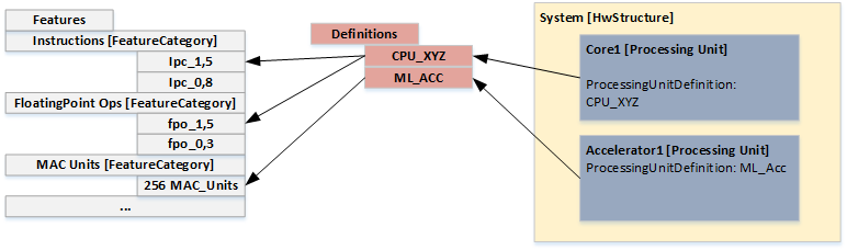
| Attribute |
Type |
Value |
Mul. |
Description |
| Name |
String |
String |
1 |
Name of the hardware feature |
| Value |
Containment |
Value |
1 |
assigned factor to the corresponding feature |
HwFeatureCategory
The
HwFeatureCategory is an element to collect the same kind of
HwFeatures with different values.
The
HwFeatureCategories can be referenced by the
ExecutionNeeds in the Software Model.
| Attribute |
Type |
Value |
Mul. |
Description |
| Name |
String |
String |
1 |
Name of the hardware feature |
| Type |
Enum |
HwFeatureType |
1 |
Type to express the purpose of the feature (performance, power, performance_and_power) |
| Description |
String |
String |
1 |
Textual description of the hardware feature |
| HwFeature |
Containment |
HwFeature |
* |
Hardware feature with a factor |
HwModule
ProcessingUnit
A
ProcessingUnit is a
HwModule that can be used to model a wide set of different hardware components like a GPU, hardware accelerator, CPU, etc. The capability and the functionality of a
ProcessingUnit are represented by different
HwFeatures within the
ProcessingUnitDefinition. The
ProcessingUnits are the master modules in the model and every
ProcessingUnit can has their own access space. The
ProcessingUnit can be referenced by
AccessPaths and
HwAccessElements.
| Attribute |
Type |
Value |
Mul. |
Description |
| Name |
String |
String |
1 |
Name of the processing unit instance |
| Ports |
Containment |
HwPort |
* |
Ports of the component |
| Caches |
Containment |
Cache |
* |
Included caches by the Processing Unit e.g. L1 Cache |
| AccessElements |
Containment |
AccessElement |
* |
Access element for a specific memory or processing unit |
| FrequencyDomain |
Reference |
FrequencyDomain |
1 |
Frequency domain which supplies the module with a frequency |
| PowerDomain |
Reference |
PowerDomain |
1 |
Power domain which supplies the module with a voltage |
| Definition |
Reference |
ProcessingUnitDefinition |
1 |
Definition with all features for the processing unit instance |
Memory
A
Memory is a component of type
HwModule to express any kind memory like SRAM (Scratchpads), DRAM, Flash, etc. in the model, caches are modeled separately. The
Memory element can be referenced as destination by a
HwAccessElement.
| Attribute |
Type |
Value |
Mul. |
Description |
| Name |
String |
String |
1 |
Name of the memory instance |
| Ports |
Containment |
HwPort |
* |
Ports of the component |
| FrequencyDomain |
Reference |
FrequencyDomain |
1 |
Frequency domain which supplies the module with a frequency |
| PowerDomain |
Reference |
PowerDomain |
1 |
Power domain which supplies the module with a voltage |
| Definition |
Reference |
MemoryDefinition |
1 |
Definition with all features for the memory instance |
Cache
A
Cache is a component of type
HwModule to express the special behavior of a
Cache. It is used to create cache topologies within a system. The
Cache can be referenced by
AccessPaths to express if it is a cached or non-cached access. It is also the only
HwModule which can be directly contained by a
ProcessingUnit.
| Attribute |
Type |
Value |
Mul. |
Description |
| Name |
String |
String |
1 |
Name of the cache instance |
| Ports |
Containment |
HwPort |
* |
Ports of the component |
| FrequencyDomain |
Reference |
FrequencyDomain |
1 |
Frequency domain which supplies the module with a frequency |
| PowerDomain |
Reference |
PowerDomain |
1 |
Power domain which supplies the module with a voltage |
| Definition |
Reference |
CacheDefinition |
1 |
Definition with all features for the cache instance |
ConnectionHandler
A
ConnectionHandler is a component of type HwModule which can be used whenever multiple
HwConnections, (HwPorts) have to be combined. It is possible to represent whole bus systems or interconnects with a single
ConnectionHandler, or elements like small routers within a NoC.
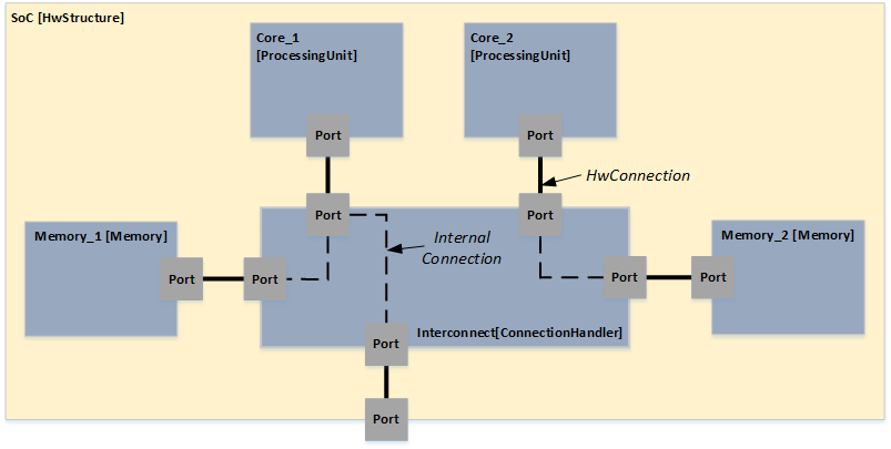
The figure shows an example where a
ConnectionHandler is used as an interconnect within a SoC. Optional it is possible to model
InternalConnections inside a
ConnectionHandler to model explicit or restrict different connections. However it is also possible to use default read and write latencies of the whole
ConnectionHandlerDefinition, individual latencies can be attached to
InternalConnections. A short example where a
ConnectionHandler is used as a CAN bus is illustrated in the structure example. For detailed models where all modules connected via
HwConnections and different
ConnectionHandlers, the
ConnectionHandlers should be the only module where contentions in the hardware model can occur. A
ConnectionHandler can be referenced by
HwAccessPaths.
| Attribute |
Type |
Value |
Mul. |
Description |
| Name |
String |
String |
1 |
Name of the connection handler instance |
| Ports |
Containment |
HwPort |
* |
Ports of the component |
| InternalConnections |
Containment |
HwConnection |
* |
Internal connection between the ports |
| FrequencyDomain |
Reference |
FrequencyDomain |
1 |
Frequency domain which supplies the module with a frequency |
| PowerDomain |
Reference |
PowerDomain |
1 |
Power domain which supplies the module with a voltage |
| Definition |
Reference |
ConnectionHandlerDefinition |
1 |
Definition with all features for the connection handler instance |
HwAccessElement
A
HwAccessElement can be used to specify the access relationship between two
ProcessingUnits or a
ProcessingUnit and a
Memory. With multiple
HwAccessElements the whole access or even address space of a
ProcessingUnit can be represented. A
HwAccessElement represents always the view from a specific
ProcessingUnit. There exist two different approaches to express latency or a data rate for a
HwAccessElement: 1. directly using latencies or data rates or 2. modeling the exact path to the destination by attaching a
HwAccessPath which references the specific connection elements like
ConnectionHandlers,
HwConnection, etc. For the second approach it is also possible to work directly with addresses.
| Attribute |
Type |
Value |
Mul. |
Description |
| Name |
String |
String |
1 |
Name of the address element |
| Destination |
Reference |
HwDestination |
1 |
Destination for the processing unit |
| AccessPaths |
Containment |
HwAccessPath |
1 |
Access path to the destination |
| ReadLatency |
Containment |
HwLatency |
1 |
Read latency to the destination |
| WriteLatency |
Containment |
HwLatency |
1 |
Write latency to the destination |
| DataRate |
Containment |
DataRate |
1 |
Max. data rate to the destination |
HwPort
HwPorts are elements which can be connected via
HwConnections. Every module can contain multiple
HwPorts. Every communication, input or output is handled via a
HwPort of a component. It is only allowed to have one
HwConnection per
HwPort, except the
HwPort is categorized as delegated port which means it is just a hierarchical connection between
HwStructures. In this case the ports can have two
HwConnections. The second exception is if inside a
ConnectionHandler,
InternalConnections are used.In this case a
HwPort can be directed with a
HwConnection and
InternalConnections. The following figure shows an example with delegated
HwPorts and
InternalConnections.
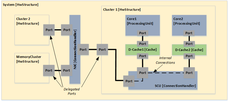
In case the
BitWidth becomes important (e.g. to calculate the amount of data which is transfered over an
ConnectionHandler) the minimum
BitWidth of all included Ports have to be accounted.
For
HwPorts it's always possible to select if the port is an
initiator or a
responder port. The following example shows that an initiator port is always connected to a responder port (comparable to TLM modeling).
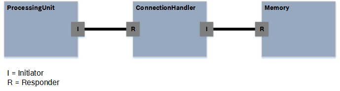
In case of a delegated port (which is used as hierarchical port at a
HwStructure) the
PortType of the module inside the structure is reflected. The following figure shows four different examples. The ports which are delegated are marked grey.
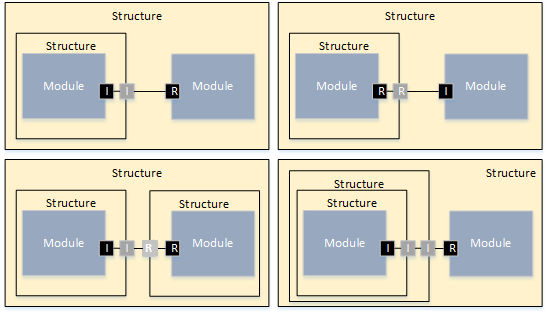
| Attribute |
Type |
Value |
Mul. |
Description |
| Name |
String |
String |
1 |
Name of the hardware port |
| BitWidth |
Int |
Int |
1 |
Bit width e.g. 32 bit (default = 0) |
| Priority |
Int |
Int |
1 |
Priority of the hardware port (default = 0) |
| Type |
Enum |
PortType |
1 |
Port type (initiator, responder) |
| Delegated |
Bool |
Bool |
1 |
Delegated ports are hierarchical structure ports |
| PortInterface |
Enum |
PortInterface |
1 |
Type to express special interfaces for validation |
HwConnection
A
HwConnection is an element to model structural connections between two
HwPorts.
HwConnections are always placed within
HwStructures. It is possible to directly annotate a read and write latency at a
HwConnection.
HwConnections can be referenced by
HwAccessPaths. The HwConnection do not have a reference to a
FrequencyDomain, the frequency is always provided by the element which is in front of the
HwConnection in the
HwAccessPath.
| Attribute |
Type |
Value |
Mul. |
Description |
| Name |
String |
String |
1 |
Name of the hardware connection |
| Port1 |
Reference |
HwPort |
1 |
Port1 for the connection |
| Port2 |
Reference |
HwPort |
1 |
Port2 for the connection |
| ReadLatency |
Containment |
HwLatency |
1 |
Constant or distribution in cycles for a read access |
| WriteLatency |
Containment |
HwLatency |
1 |
Constant or distribution in cycles for a write access |
| DataRate |
Containment |
DataRate |
1 |
Max. data rate of the connection (value and unit) |
HwAccessPath
A
HwAccessPath is an element to describe the connection route of a
ProcessingUnit to its destination (
Memory or
ProcessingUnit). The
HwAccessPath is defined through an ordered list of IPaths interface elements (
HWConnections, Caches and
ConnectionHandlers) and is a containment of an
HwAccessElement. The figure shows an example of an
HwAccessPath, how a
ProcessingUnit is connected via two
HwConnections and a
ConnectionHandler with a
Memory.
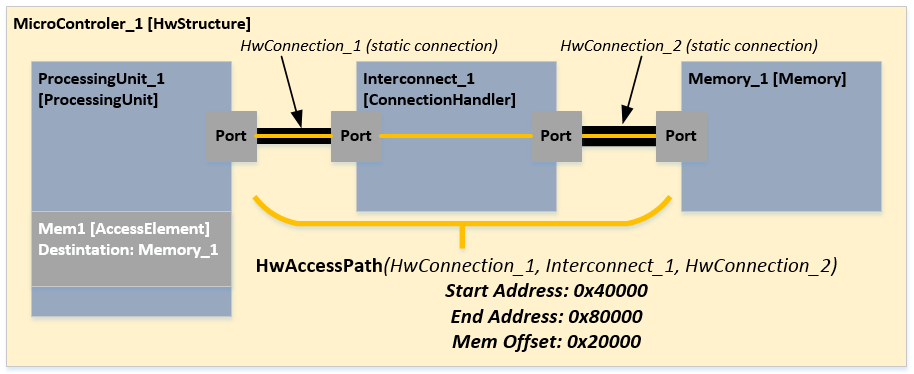
In the following example the possible memOffset attribute is explained. Every
ProcessingUnit can access a
Memory or other
ProcessingUnit over a different address. The size of the
Memory has to be equal or greater than
endAddress minus the
startAddress.
- memory_size >= endAddress – startAddress
In the case the the
ProcessingUnit should not start at address 0 (from the memory point of view) the
memOffset attribute can be used. With help of this attribute the access area for the memory can be changed, the following figure shows an example.
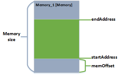
| Attribute |
Type |
Value |
Mul. |
Description |
| Name |
String |
String |
1 |
Name of the hardware access path |
| PathElements |
Reference |
HwPath |
* |
Path elements for the access path |
| StartAddress |
Long |
Long |
1 |
Start address for the memory |
| EndAddress |
Long |
Long |
1 |
End address for the memory |
| MemOffset |
Long |
Long |
1 |
Offset for accessing only a partition of a memory |
Enumerations
In the following all enums are listed. In the case an enum is used by any class the default value of that enum is always
undefined. That means that in case of an enum there are no default values for interfaces or other kind of types. Moreover only new enums are explicitly mentioned in this report. Enums and classes which are already part of the existing Amalthea meta model are not described.
StructureType:
- _undefined_, System, ECU, Microcontroller, SoC, Cluster, Group, Array, Area, Region
CacheType:
- _undefined_, instruction, data, unified
VoltageUnit:
PortType:
- _undefined_, initiator, responder
SchedPolicy:
- _undefined_, RoundRobin, FCFS, PriorityBased
WriteStrategy:
- _undefined_, none, writeback, writethrough
PuType:
- _undefined_, GPU, CPU, Accelerator
PortInterfaces:
- _undefined_, custom, can, flexray, lin, most, ethernet, spi, i2c, axi, ahb, apb, swr
HwFeatureType:
- _undefined_, performance, power, performance_and_power
MemoryType:
- _undefined_, DRAM, SRAM, FLASH, PCM
3.9 Mapping Model
The mapping model is intended to provide tools that use hardware and software models (e.g. code generators) information about the corresponding mappings and allocations. This information contains associations between
- schedulers and executable software: A scheduler manages and distributes executable software like runnables or tasks on its managed processing units
- schedulers and processing units: A scheduler can manage one or more processing units and deploy computations on these
- data and memories: Data (such as functions, variables, heap etc) is mapped on static and volatile memories
Note the mapping model is the only sub model of Amalthea with an attribute in the root element. The
Address Mapping Type defines the interpretation of used addresses in the mapping model. Additional information can be found in the
MemoryMapping section.
The Meta Model specifying the Mapping Model is shown below.

MappingModel
The
MappingModel serves as a container for each of the mapping rules, i.e.
Allocations (executable software and processing units which are allocated to schedulers) and
Mappings (labels and software which is mapped to memories).
3.9.2 Allocations

SchedulerAllocation
The
SchedulerAllocation describes the allocation of a
Scheduler to processing units. This class consists of references to the respective
Scheduler, which is specified within an existing OS model, and a processing units, which is specified in a hardware model. Schedulers with algorithm "Grouping" are not allocated since they take no decisions and produce no overhead.
| Name |
Description |
|
scheduler
|
The scheduler (that is specified in more detail). |
|
responsibility
|
Defines the processing units the scheduler is responsible for. On these units the scheduler takes decisions. Multiple schedulers can be responsible for one processing unit because of hierarchies. Child-schedulers only take decisions, if they parent-schedulers allows them to (e.g. hypervisors with virtual machines which execute an own operating system). Tasks allocated to this scheduler execute on the intersection between affinity and the responsibility of the scheduler. If this is null the configuration is invalid. If the intersection results in multiple cores, the task can migrate. |
|
executingPU
|
Defines on which processing unit the scheduling algorithm is actually executed to consider the overhead. |
RunnableAllocation
The
RunnableAllocation is used to associate a
Runnable, specified within an existing software model, with a
Scheduler.
TaskAllocation
The
TaskAllocation is used to associate a
Task with its
TaskScheduler.
| Name |
Description |
|
task
|
The task (that is specified in more detail). |
|
scheduler
|
Specifies the unique allocation to the scheduler of the task. |
|
affinity
|
Specifies the possible processing units the task can run. If only one unit is specified, the task runs on this core. If multiple cores are specified, the task can migrate between the units. The task executes on the intersection between affinity and the responsibility of the scheduler. If this is null the configuration is invalid. If the intersection results in multiple cores, the task can migrate. |
|
schedulingParameters
|
Used to assign scheduling parameters for this specific allocation. For details see chapter "Scheduling Parameters" in OS Model. |
ISRAllocation
The
ISRAllocation is used to associate an
ISR with an
InterruptConroller. The attribute 'priority' can be used to assign a value for this specific allocation.
MemoryMapping
The
MemoryMapping is a class, describing the mapping of parts of the software model to
Memory. It is used to associate specializations of the
AbstractMemoryElement (i.e.
Label,
Runnable,
TaskPrototype and
Process). The target memory is specified by a reference to an explicit
Memory within an existing hardware model. The position in memory can also be defined as address here. If the address is a absolute memory address, a offset address from the memories first address, or if the address information is not expected at all is defined by the
Memory Address Mapping Type enumeration in the root element of the
Mapping Model. The Additional attributes, e.g. to supply further information for a code generator, may be described by the containment attributeList.
PhysicalSectionMapping
The
PhysicalSectionMapping class (can also be called as
Physical Memory Section ) describes the following:
- mapping of various
Section elements to a specific
Memory
- mapping various
Label and Runnable elements to a Physical Memory Section
- description of memory address location where the Physical Memory Section is allocated
Note for additional information (see User Guide > Concepts > Memory Sections)
3.10 OS Model
This part of the AMALTHEA model describes the provided functionality of an operating system. Therefore the concepts of scheduling, overheads, and semaphores are supported, which are described in detail in the following chapter.

3.10.1 Operating System
The basic element in the OS Model is the operating system. There can be multiple operating systems in one model. The operating system type can be used to describe a generic operating system. It is also possible to use the vendor operating system type to define a vendor specific OS. An operating system contains a number of task schedulers and interrupt controllers. A task scheduler controls the execution of a task on one or multiple processor cores. An interrupt controller is the controller for the execution of ISRs and can be also mapped to multiple cores. The mapping of tasks and ISRs to their controller and the mapping of the controller to the cores can be done in the Mapping Model. An operating system can also contain a description of the overhead it produces. For this there is a more detailed explanation below.
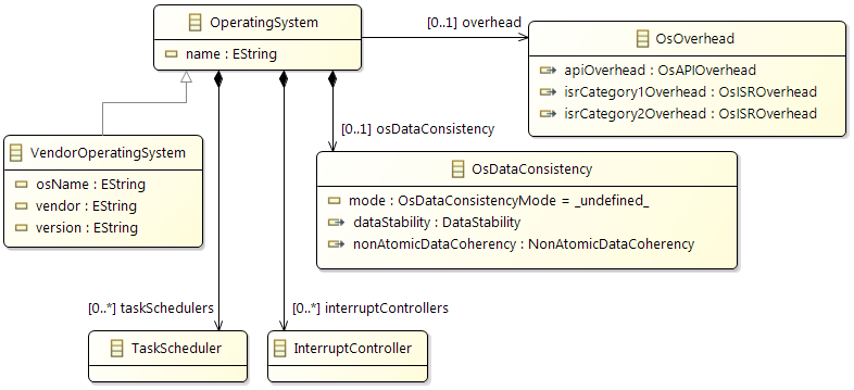
3.10.2 Scheduler, Scheduler Definitions, and their Parameters
Schedulers refer to a
definition which specifies the scheduling algorithm that decides if and when to schedule a processes. Each scheduler definition may refer to algorithm and process parameters (type is a
SchedulingParameterDefinition). Algorithm parameters are set per scheduler whereas process parameters may have different values per process allocation (task or ISR). Each scheduler can have
schedulingParameters which assign values to the algorithm parameters of their definition, i.e., a deferrable server scheduler should have a value for the algorithm parameter
capacity. Schedulers can have computation items (a subset of the runnable items) that characterize the runtime behavior (algorithmic overhead) of the scheduler.

There are additional attributes in the scheduler definition to define the behavior of the scheduler in a hierarchy (parent and child schedulers):
| Name |
Description |
|
requiresParentScheduler
|
boolean attribute indicating whether the scheduler requires a parent scheduler, defaults to
false.
|
|
passesParametersUpwards
|
boolean attribute that specifies that scheduler parameters set for a
TaskAllocation will be passed on to the parent scheduler (if this scheduler does not have a parameter with this name), defaults to
false.
|
|
hasExactlyOneChild
|
boolean attribute that indicates if the scheduler can schedule only one schedulable entity or if it can schedule multiple ones, defaults to
false.
|
Scheduler Definition
A scheduler definition is contained in the OS Model. There may be multiple scheduler definitions in the model. The definition has a name which is also used to uniquely identify standard scheduler definitions (like OSEK, EarliestDeadlineFirst, etc.) There is a number of standard scheduler definitions that are known in AMLATHEA they can be added automatically to each model and should not be changed. Scheduler definitions refer to algorithm and process parameters. Algorithm parameters can be set for each scheduler that uses the scheduler definition. Process parameters can be set for scheduler associations or task allocations.
Scheduling Parameter Definition and Scheduling Parameter
Scheduling parameter definitions are contained in the OS Model an may be referred to by multiple scheduler definitions. They have a type, can consist of many values (default is false), can be mandatory (default is true), and may provide a default value that shall be used if they are not mandatory. Scheduling parameters are key value pairs where the key is the definition and the value is some literal of type
Value. The type specified in the scheduling parameter definition dictaes possible literals of their value, e.g. type
Integer allows
BigInteger,
long, and
integer literals. Standard scheduler definitions have only
mandatory parameters (if there is no default value provided).

Standard Scheduler Definitions
The following gives a tabular overview of the standard scheduler definitions supported by AMLATHEA. The user can also define custom schedulers and parameters, but they may not be supported by tools importing AMALTHEA models.
| Scheduling Algorithm |
Description and Parameters |
| Fixed Priority |
|
OSEK
|
OSEK compliant Scheduling. A fixed priority preemptive scheduling algorithm with task groups. Tasks belonging to the same task group are scheduled cooperatively (they do not preempt each other), preemptive otherwise. Tasks with the same priority also behave cooperatively. |
| Process parameters |
priority [1] Integer: The priority of the process (a higher value means a higher priority).
|
|
taskGroup [1] Integer: The OSEK task group number (if for two processes the number is equal, that means they are in the same task group).
|
|
FixedPriorityPreemptive
|
Fixed Priority Preemptive Scheduling (e.g. AUTOSAR), same as OSEK but without task groups. |
| Process parameters |
priority [1] Integer: The priority of the process (a higher value means a higher priority).
|
| Dynamic Priority |
|
EarliestDeadlineFirst
|
Earliest Deadline First (EDF): Task with the closest deadline in relation to the current point in time will be scheduled next. First introduced in: Liu, Chung Laung, and James W. Layland. "Scheduling algorithms for multiprogramming in a hard-real-time environment." Journal of the ACM (JACM) 20.1 (1973): 46-61. |
| Process parameters |
deadline [1] Time: The time after each activation at which the process must finish.
|
|
PriorityBasedRoundRobin
|
Round Robin scheduling algorithm assignes equally sized time slices to each process that it schedules. The priority describes the order in which the processes will be executed. If two processes have the same priority, the order of these two is random (non-deterministic). |
| Algorithm parameters |
timeSliceLength [1] Time: Length of each time slice.
|
| Process parameters |
priority [1] Integer: The priority of the process (a higher value means a higher priority).
|
| Proportionate Fair (Pfair) |
|
PfairPD2
|
Proportionate Fair PD2 Scheduling (Pfair-PD2) |
| Algorithm parameters |
quantSize [0..1] Time = 1ns: Length of the minimum schedulable time slot used in Pfair scheduling. It is assumed that execution times are an integer multiple of this time slot length.
|
|
PartlyPfairPD2
|
Partly Proportionate Fair PD2 Scheduling (PPfair-PD2) |
| Algorithm parameters |
quantSize [0..1] Time = 1ns: Length of the minimum schedulable time slot used in Pfair scheduling. It is assumed that execution times are an integer multiple of this time slot length.
|
|
EarlyReleaseFairPD2
|
Early Release Fair PD2 Scheduling (ERfair-PD2) |
| Algorithm parameters |
quantSize [0..1] Time = 1ns: Length of the minimum schedulable time slot used in Pfair scheduling. It is assumed that execution times are an integer multiple of this time slot length.
|
|
PartlyEarlyReleaseFairPD2
|
Partly Early Release Fair PD2 Scheduling (P-ERfair-PD2) |
| Algorithm parameters |
quantSize [0..1] Time = 1ns: Length of the minimum schedulable time slot used in Pfair scheduling. It is assumed that execution times are an integer multiple of this time slot length.
|
| Reservation Based Server |
|
GroupingServer
|
This is not a scheduler algorithm. Schedulers using this definition act as a logical grouping of tasks/child-schedulers, e.g. a partition for some tasks for budget accounting reasons. This scheduler does not take any scheduling decisions, and a parent scheduler is mandatory. |
| Algorithm parameters |
capacity [1] Time: The fixed budget that can be used by processes. It will be replenished periodically.
|
|
period [1] Time: Amount of time after which the capacity will be replenished.
|
| Definition attributes |
☑ requires parent scheduler
☑ passes parameters upwards
☐ has exactly one child |
|
DeferrableServer
|
Deferrable Server (DS): provides a fixed budget, in which the budget replenishment is done periodically. First introduced in: Strosnider, Jay K., John P. Lehoczky, and Lui Sha. "The deferrable server algorithm for enhanced aperiodic responsiveness in hard real-time environments." IEEE Transactions on Computers 44.1 (1995): 73-91. |
| Algorithm parameters |
capacity [1] Time: The fixed budget that can be used by processes. It will be replenished periodically.
|
|
period [1] Time: Amount of time after which the capacity will be replenished.
|
| Defintion attributes |
☑ requires parent scheduler
☐ passes parameters upwards
☑ has exactly one child |
|
PollingPeriodicServer
|
Polling Server (PS): provides a fixed budget periodically that is only available at pre-defined times. If the process is not using the budget at that point in time the budget is lost. |
| Algorithm parameters |
capacity [1] Time: The fixed budget that can be used by processes (usually directly after it has been replenished). The capacity will be consumed even if there is no process using it. It will be replenished periodically.
|
|
period [1] Time: Amount of time after which the capacity will be replenished.
|
| Defintion attributes |
☑ requires parent scheduler
☐ passes parameters upwards
☑ has exactly one child |
|
SporadicServer
|
Sporadic Server (SS): provides a fixed budget, in which the budget replenishment is performed with a pre-defined replenishment delay after it was consumed. First introduced in: Sprunt, Brinkley, Lui Sha, and John Lehoczky. "Aperiodic task scheduling for hard-real-time systems." Real-Time Systems 1.1 (1989): 27-60. |
| Algorithm parameters |
capacity [1] Time: The fixed budget that can be used by processes. It will be replenished after the specified amount of time has passed since it has last been consumed.
|
|
replenishmentDelay [1] Time: Amount of time after which the capacity will be replenished after it has last been consumed.
|
| Defintion attributes |
☑ requires parent scheduler
☐ passes parameters upwards
☑ has exactly one child |
|
ConstantBandwidthServer
|
Constant Bandwidth Server (CBS): provides a fixed utilization for executing jobs, in which the deadline for execution is independent on the execution time of jobs. First introduced in: Abeni, Luca, and Giorgio Buttazzo. "Integrating multimedia applications in hard real-time systems." Proceedings 19th IEEE Real-Time Systems Symposium (Cat. No. 98CB36279). IEEE, 1998. |
| Algorithm parameters |
capacity [1] Time: The fixed budget that can be used by processes. It will be replenished periodically.
|
|
period [1] Time: Amount of time after which the capacity will be replenished.
|
| Defintion attributes |
☑ requires parent scheduler
☐ passes parameters upwards
☑ has exactly one child |
|
ConstantBandwidthServerWithCapacitySharing
|
Constant Bandwidth Server (CBS) with capacity sharing (CASH). Consumes residual slack from other servers (work conserving). |
| Algorithm parameters |
capacity [1] Time: The fixed budget that can be used by processes. It will be replenished periodically.
|
|
period [1] Time: Amount of time after which the capacity will be replenished.
|
| Defintion attributes |
☑ requires parent scheduler
☐ passes parameters upwards
☑ has exactly one child |
Further information
Details regarding proportionate fair (
Pfair) scheduling and the variants of the
PD2 Pfair algorithm can be found in the dissertation "Effcient and Flexible Fair Scheduling of Real-time Tasks on Multiprocessors" by Anand Srinivasan (see
dissertation at University of North Carolina at Chapel Hill).
An overview regarding
Reservation Servers is given in the lecture "Resource Reservation Servers" by Jan Reineke (see
lecture at Saarland University).
Scheduler Association
A hierarchy of schedulers can be specified with intermediate objects of class
SchedulerAssociation. If set, the parent scheduler takes the initial decision who is executing. If the child-scheduler is not a grouping of tasks, it can take scheduling decisions if permission is granted by the parent. The association also contains the relevant scheduling parameters for the scheduler in the hierarchical context.

| Attribute |
Description |
|
parent
|
Refers to the parent scheduler |
|
child
|
Derived attribute that is computed based on the containment reference "parentAssociation" from
Scheduler to
SchedulerAssociation
|
|
schedulingParameters
|
See chapter "Scheduling Parameters" |
It is possible to define the overhead that is produced by an operating system. The defined overhead can be assigned to an operating system definition. Each overhead information is defined as a set of instructions that has to be executed when the corresponding OS function is used. The instructions can be either a constant set or a deviation of instructions. It is possible to define the overhead for the ISR category one and two and for a number of operating system API functions.
ISR Overhead
- ISR category 1 & 2: Describes the overhead for ISRs of category one and two by adding a set of instructions that is executed at start and terminate of the ISR
API Overhead
There exists also an overhead for API calls. The following API calls are considered:
- API Activate Task: Runtime overhead for the activation of a task or ISR by another task or ISR (inside the activating process)
- API Terminate Task: Runtime for explicit task termination call (inside a task)
- API Schedule: Runtime for task scheduling (on scheduling request)
- API Request Resource: Runtime overhead for requesting a semaphore (inside a runnable)
- API Release Resource: Runtime overhead for releasing a semaphore (inside a runnable)
- API Set Event: Runtime overhead for requesting an OS event (inside a task or ISR)
- API Wait Event: Runtime overhead for waiting for an OS event (inside a task or ISR)
- API Clear Event: Runtime overhead for clearing an OS event (inside a task or ISR)
- API Send Message: Runtime overhead for cross-core process activation or event (inside a task or ISR)
- API Enforced Migration: Runtime overhead for migrating from one scheduler to another scheduler (inside a task or ISR)
- API Suspend OsInterrupts
- API Resume OsInterrupts
- API Request Spinlock
- API Release Spinlock
- API SenderReceiver Read
- API SenderReceiver Write
- API SynchronousServerCallPoint
- API IOC Read
- API IOC Write
3.10.4 OS Data Consistency
The
OsDataConsistency class provides a way to configure an automatic data consistency mechanism of an operating system. It is used to cover the following two use cases:
- Provide a configuration for external tools that perform a data consistency calculation based on the stated information.
- Provide the results of a performed data consistency calculation which then have to be considered by external tools (e.g. by timing simulation).
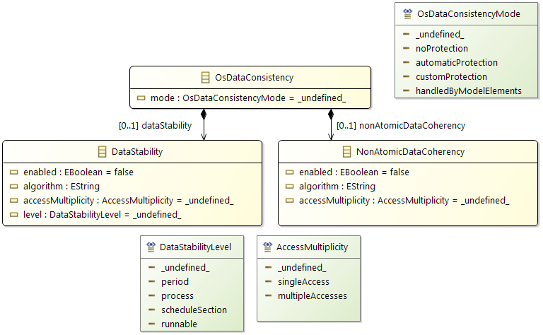
To distinguish the different use cases and to consequently also indicate the workflow progress for achieving data consistency,
OsDataConsistencyMode allows to define the general configuration of the data consistency. The following modes are available:
- noProtection: data stability and coherency is NOT automatically ensured.
- automaticProtection: data stability and coherency HAS TO BE ensured according configuration either via custom protection or via model elements.
- customProtection: data stability and coherency IS ensured according configuration but not via model elements.
- handeldByModelElements: data stability and coherency IS ensured via model elements.
The
DataStability class defines for which sequence of runnables data has to be kept stable. Furthermore, it can be stated whether all data is considered for stability or just those accessed multiple times.
DataStabilityLevel:
-
period - between consecutive activations
-
process - within a Task or ISR
-
scheduleSection - between Schedule points (explizit schedule points, begin and end of process)
-
runnable - within a Runnable
The
NonAtomicDataCoherency class defines for which sequence of runnables data has to be kept coherent. Like for data stability it can be stated whether all data is considered for coherency or just those accessed multiple times.
With this object, a semaphore or locking mechanism can be described which restricts the access of several processes to one resource at the same time.
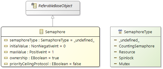
| Attribute |
Description |
|
name
|
Name of semaphore (inherited from ReferableBaseObject) |
|
semaphoreType
|
Defines how the semaphore is implemented (see below) |
|
initialValue
|
Initial number of already used/locked resources |
|
maxValue
|
Maximum possible number of available locks/resources |
|
ownership
|
Defines if the lock can only be released by the process that acquired it |
|
priorityCeilingPrototcol
|
Defines if the priority ceiling protocol is activated. If it is activated, a process that accesses the semaphore gets a higher priority as the processes that can also access the same semaphore |
The different types of semaphores are summarized in the following table. For the ownership there are two possibilities: true – central (only the process that acquired the lock can release it), false – decentral (any process can release it). The priority ceiling property specifies whether the locking mechanism can be used with the priority ceiling protocol to avoid priority inversion, or not. The waiting behavior specifies how a requesting process is allowed to wait for the lock (during a SemaphoreAccess, see Software Model). The access type specifies how different access types will be interpreted, i.e., spinlocks can only be requested exclusively, since there is only one lock.
| Semaphore type |
Description & Properties |
|
CountingSemaphore
|
This locking mechanism enables multiple processes to concurrently access the semaphore. The number of allowed concurrent accesses is specified by
maxValue. Since counting semaphores can be released by processes other than the ones that acquired it, the priority ceiling protocol can not be applied. Additionally, an exclusive access means that the requesting process waits until all counting semaphores are available and will acquire all of them. The next release access will then release all counting semaphores.
|
| value specification |
initial: 0..N (already locked); range: 0..N |
| ownership |
true/false, central/decentral |
| priority ceiling |
false |
| waiting behavior |
active/passive |
| access type |
request, exclusive, release |
|
Resource
|
A resource is similar to a counting semaphore. Multiple concurrent accesses are allowed up to
maxValue. However, since ownership is required, only processes that acquired the resource before can release it. The priority ceiling protocol can also be applied if needed. An exclusive access means the same as for counting semaphores, albeit with the ownership restriction.
|
| value specification |
initial: 0 (all available); range: 0..N |
| ownership |
true, central: Process |
| priority ceiling |
true/false |
| waiting behavior |
active/passive |
| access type |
request, exclusive, release |
|
Spinlock
|
Spinlocks can be used like a resource with
maxValue =1, however, only active waiting is supported during a request access. Since there is only one spinlock, any request is always exclusive.
|
| value specification |
initial: 0 (unlocked); range: 0..1 |
| ownership |
true, central: Process |
| priority ceiling |
true/false |
| waiting behavior |
active only |
| access type |
request = exclusive, release |
|
Mutex
|
Mutexes (MUTual EXclusive lock access) are very similar to spinlocks. As opposed to spinlocks, processes can also passively wait until they are available. Again, requests are always exclusive. |
| value specification |
initial: 0 (unlocked); range: 0..1 |
| ownership |
true, central: Process |
| priority ceiling |
true/false |
| waiting behavior |
active/passive |
| access type |
request = exclusive, release |
-
Semaphore: The
initialValue must not be greater than the
maxValue!
-
Semaphore: The
initialValue must be 0 for
Resource,
Spinlock, or
Mutex!
-
Semaphore: The
ownership must be
true for
Resource,
Spinlock, or
Mutex!
-
Semaphore: The
maxValue must be 1 for
Spinlock or
Mutex!
-
Semaphore: The
priorityCeilingProtocol must be
false for
CountingSemaphore!
3.11 PropertyConstraints Model
The scope of the Property Constraints model is to limit the design space by providing information about the specific hardware properties that parts of the software rely on, i.e. what properties or features have to be supplied by the respective hardware in order to be a valid mapping or allocation target.
This information comprises
- Core allocation constraints, which describe the constraints on cores.
- Memory mapping constraints, which describe the constraints on memories.
The figure below shows the Property Constraints model. In order to provide a better understanding of the model, interconnections between software model elements are not shown in this figure.
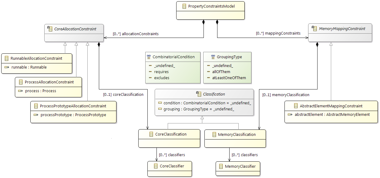
3.11.2 CoreAllocationConstraint
The
CoreAllocationConstraint is an abstract class for describing constraints which affect the selection of a suitable
Core.
RunnableAllocationConstraint
The
RunnableAllocationConstraint is a specialization of the
CoreAllocationConstraint. It is used to specify constraints on
Core elements which are used in
Runnable to
Core allocations.
ProcessAllocationConstraint
The
ProcessAllocationConstraint is a specialization of the
CoreAllocationConstraint. It is used to specify constraints on
Core elements which are used in the allocation of Process's specializations (i.e.
Task and
ISR), to
Cores.
ProcessPrototypeAllocationConstraint
The same as ProcessAllocationConstraint but for process prototypes in an earlier phase of the development.
3.11.3 MemoryMappingConstraint
The
MemoryMappingConstraint is an abstract class for describing constraints which affect the selection of a suitable
Memory. The actual constraint on the core is described by the
AbstractElementMappingConstraint.
AbstractElementMappingConstraint
The
AbstractElementMappingConstaint is a specialization of the
MappingConstraint. It is used to specify constraints on
Memory elements which are used in the mapping of
AbstractMemoryElement specializations (i.e.
Label,
Runnable,
TaskPrototype or
Process) to
Memories.
3.11.4 Classifications
The specializations
CoreClassification and
MemoryClassification are used to describe the features that a hardware element (
Core or
Memory) needs to provide in order to be a valid target. This is done by references to Classifiers, conditions (requires vs. excludes) and the kind of grouping (all of them vs. at least one of them).
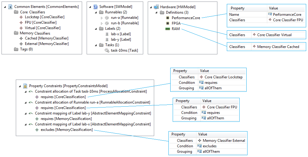
3.12 Stimuli Model
The Stimuli Model contains stimulus and clock objects.
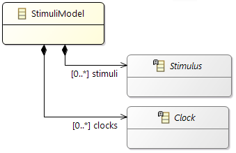
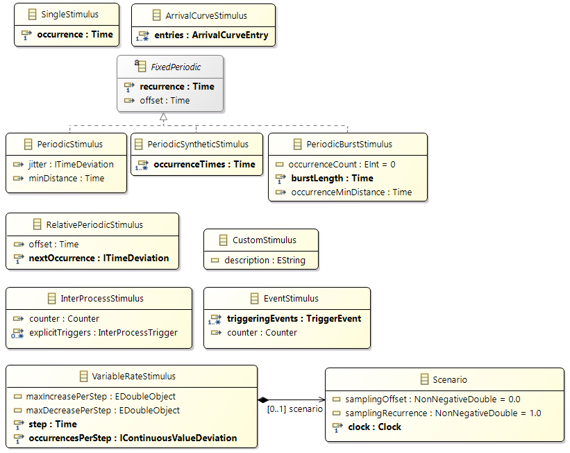
A stimulus is responsible to activate processes. The following different types are available:
-
SingleStimulus: Activates the process only once.
-
ArrivalCurveStimulus: A list of time-borders in which a specified number of occurrences are expected.
-
PeriodicStimulus: Periodic activations based on an offset, a recurrence and (optionally) a jitter.
-
PeriodicSyntheticStimulus: Defines a periodically triggered stimuli depending on a defined list of occurrence times.
-
PeriodicBurstStimulus: Defines a periodic burst pattern of the process.
-
RelativePeriodicStimulus: Periodic activation based on offset and a recurrence.
In contrast to PeriodicStimulus the recurrence is relative to the last occurrence and a deviation is mandatory.
-
VariableRateStimulus: Periodic activations based on other events, like rotation speed.
-
InterProcessStimulus: Activations based on an explicit inter-process activation.
Contains a Counter element if activation is either shifted and / or happening every nth time.
-
EventStimulus: Activation triggered by an event, defined in the event model.
Contains a Counter element if activation is either shifted and / or happening every nth time.
-
CustomStimulus: To describe own custom types of activations, including properties.
-
PeriodicStimulus: The
Time object in the role of
offset must not contain a negative value!
-
PeriodicStimulus: The
Time object in the role of
recurrence must not contain a negative value!
-
PeriodicBurstStimulus: The
Time object in the role of
offset must not contain a negative value!
-
PeriodicBurstStimulus: The
Time object in the role of
recurrence must not contain a negative value!
-
PeriodicSyntheticStimulus: The
Time object in the role of
offset must not contain a negative value!
-
PeriodicSyntheticStimulus: The
Time object in the role of
recurrence must not contain a negative value!
-
TimestampList: The
Time objects in the role of
timestamps must not contain a negative value!
-
SingleStimulus: The
Time object in the role of
occurrence must not contain a negative value!
-
ArrivalCurveEntry: The
Time object in the role of
lowerTimeBorder must not contain a negative value!
-
ArrivalCurveEntry: The
Time object in the role of
upperTimeBorder must not contain a negative value!
Single
Single allows to specify an activation at a single relative point in time. The single activation occurs after the time units specified by
occurrence.
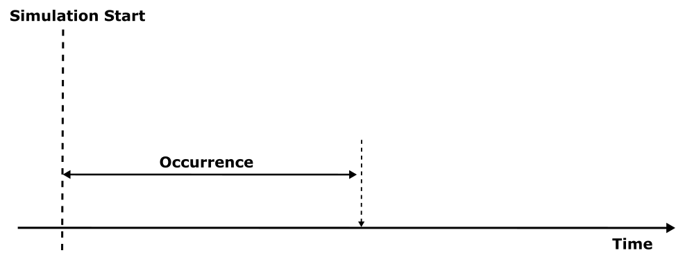
Arrival Curves
An arrival curve is described as a list of time-borders in which a specified number of activations are expected. The picture below shows an example for this. In the first picture there is a number of occurrences on a timeline.
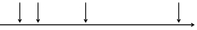
In the picture below every distance between two activations is measured. The minimum and the maximum distance is added to the table as time-border for the occurrence of two activations. This means that after one activations there has to be at least a gap of one time-unit before the next activations can occur. It also means that there will be always a second activations within eight time units after the last activations. Basically this would be enough to describe an Arrival Curve Stimulus. But it is possible to create a more precise stimulus by describing additional time borders for greater number of occurrences. This is shown in the steps below.
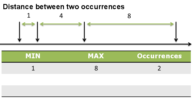
The same as for two activations in the picture above is done here for three activations. Like already mentioned above, this is an additional restriction for occurrence of an activations.
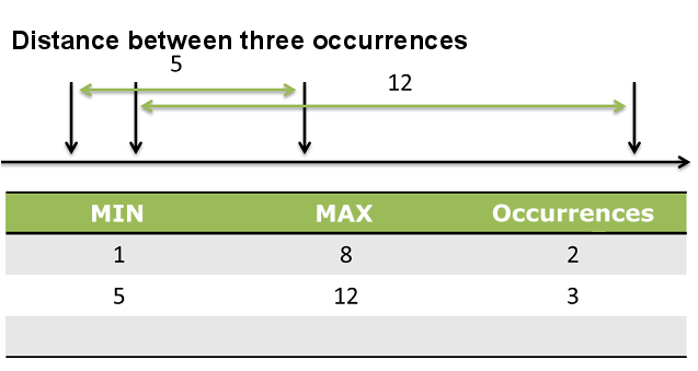
And for four activations:
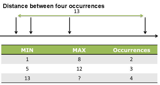
The picture below shows the table as arrival curve graph. The red line is the upper-time-border that shows the latest time where the activations will occur. The green line shows the earliest possible time where the activations can occur.
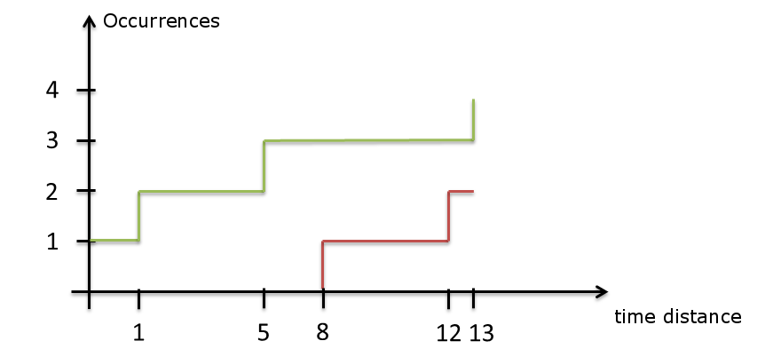
Common properties of fixed periodic stimuli
The abstract class
FixedPeriodic defines the common attributes of
Periodic,
PeriodicSynthetic and
PeriodicBurst. In general all period based Stimuli specify periodic occurrences based on an offset and a recurrence. The first occurrence happens after the time units specified by
offset, and then every following occurrence happens after the time units specified by
recurrence. This means, in general, an occurrence of instance i is happening at time t =
offset + i *
recurrence.
The following figure shows a
Periodic Stimulus example with only a fix offset and recurrence time.
Periodic
In addition to the standard periodic behavior the
Periodic Stimulus can be extended by a
Jitter e.g. an Gaussian deviation. The activation time of each occurrence jitters according to the values of the distribution as depicted in the following figure. Depending on the
Jitter distribution the upper bound of the current and the lower bound of the next activation can be close to each other or even overlap. The
minDistance value allows the user to define the minimum distance between the current and the next activation.
The recurrence of a
Periodic Stimulus is absolute. This means that a recurrence of 10ms points exactly to the next activation every 10ms. The
Jitter describes the deviation of the occurrence around this absolute value.
PeriodicSynthetic
PeriodicSynthetic allows to specify a periodic activation of trigger patterns. It is defined by a list of List of
occurrenceTimes, a period
recurrence, and an
offset. Each time value in
occurrenceTimes specifies a single activation at a relative point in time. The moment in time these time values are relative and is defined the following way: an activation of instance i is triggered at time t =
offset + floor(i / m) *
recurrence +
occurrenceTimes[i modulo m].
The following figure shows a
Synthetic Stimulus example with two periodic activations after the time units T1 and T2.
PeriodicBurst
The
PeriodicBurst Stimulus specifies a set of burst activations that are periodically repeated. This means that multiple activations occur very close to each other and this recurs in a periodic matter. The burst pattern has a fixed recurrence period and every burst results in multiple activations.
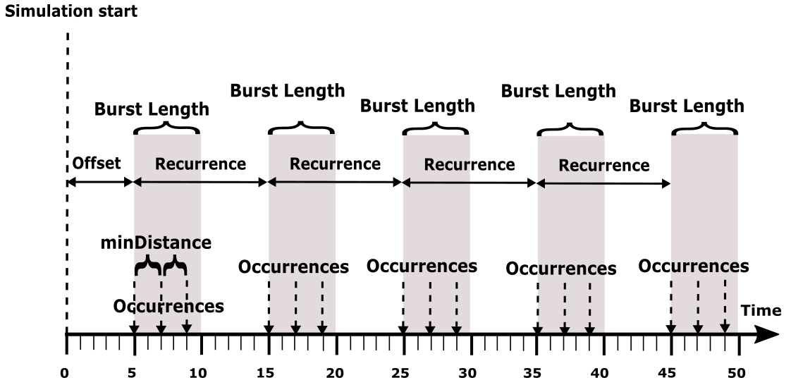
The number of occurrences per burst are specified via
occurrenceCount. The
occurrenceMinDinstance defines the minimal distance between them. The
burstLength defines the maximum time the burst pattern can last. If (number of occurrences – 1) multiplied with the minimum distance between activations is bigger than the
burstLength only the number of activations that fit into the
burstLength are executed.
RelativePeriodic
In contrast to the
Periodic Stimulus the
RelativePeriodic Stimulus allows to specify relative recurrences. The next activation depends on the current activation time and the added deviation for the next step. The
lower and
upperBound are specified in the
nextOccurrence deviation similar to the
Jitter specification in the
Periodic Stimulus.
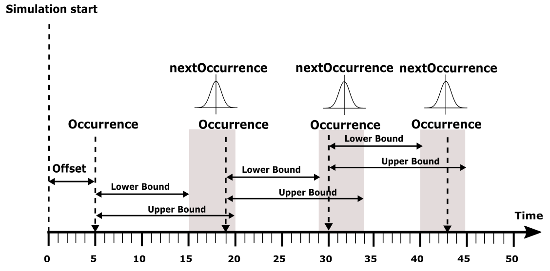
VariableRateStimulus
With the
VariableRate Stimulus the description of task activation based on e.g. the crankshaft rotation speed or other adaptive variable rate activations.
The
step has to be defined as a base value for the following specifications.
In the deviation
occurrencesPerStep the lower and upper frequency of the variable rate are described. The distribution can be used to describe the standard frequency occurrences. The user can describe that the frequency is distributed e.g. uniformly over the complete frequency band or as another example the occurrences happens mostly at the
Boundaries of the frequency band that can be specified with the
CornerCase
samplingType in the distribution.
The user can set
maxDecrease and
maxIncrease values to describe the number of additional respectively reduced task activations that can occur within a predefined time
step. With these values, the maximum acceleration and maximum deceleration of the stimuli can be calculated.
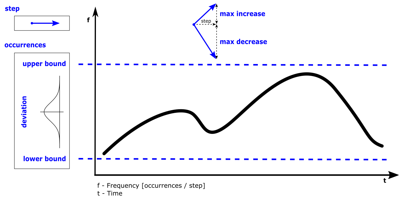
An additional feature for the
variableRate Stimulus is the description of
simulationScenario that specifies the progression of the
variableRate over time.
In contrast to the generic specification via statistical values the scenario defines the computation via the
samplingOffset and
samplingRecurrence property that is modified by a factor based on a
clock.
The
Clock is triggered based on logical clocks rather than the simulation time, thus providing a dynamic trigger pattern for a simulation.
Clock defines the (variable) rate at which a stimulus will be fired. This rate follows a certain pattern defined by the subclasses:
ClockFunction and
ClockStepList.
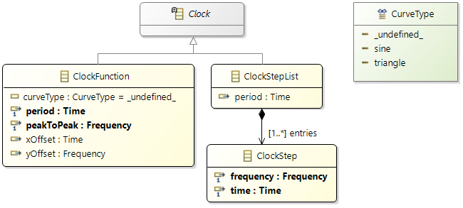
ClockFunction
A clock function defines the clock period change via a continuous function. There are two functions available:
Sine and
Triangle. They can be chosen by setting the
curveType property.
In the sine clock function the clock period increases and decreases smoothly following a sine wave pattern. The figure below depicts the attributes used to define the sine wave. Note that the sine wave always lies above the x-axis. Adding a positive or negative
x-Offset will shift the wave horizontally. The clock fires a stimulus whenever the area under the sine curve is a multiple of one (an integral value). If used in a
Scenario this factor can be defined via the
samplingRecurrence attribute. As can be seen, the size of the area can be influenced by the
yOffset and
peakToPeak attributes. In the example shown in the figure the first stimulus is fired at 1.3s, second at 2.06s and so on.
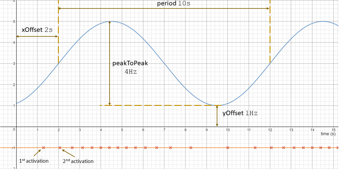
The triangle clock function increases and decreases at a constant rate. The shape of this clock function is governed by the same attributes as the sine wave, only the underlying mathematical definition is different. In the example figure below, the first activation occurs at 0.828s, the second at 1.464s and so on.
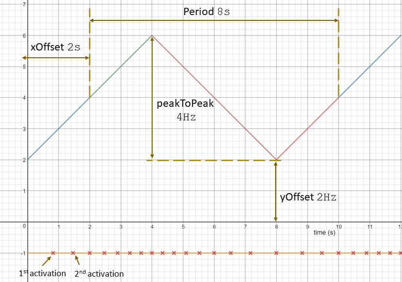
ClockStepList
The list of clock steps defines the clock period change via a step function. Each
ClockStep of that function is defined by a
frequency and a
time stamp. The optional period attribute of the clock step list can be used to repeat the pattern (exactly like the recurrence in the
PeriodicSynthetic stimulus). If the period is not set, the clock rate will remain the same after the last clock step change. Considering the clock steps: <1Hz, 1s>, <3Hz, 3s>, <2Hz, 5s>, <0Hz, 6s>, <2Hz, 7s>, a sampling recurrence of 2, and a period of 9s, the clock step function will result in the plot depicted in the following figure.
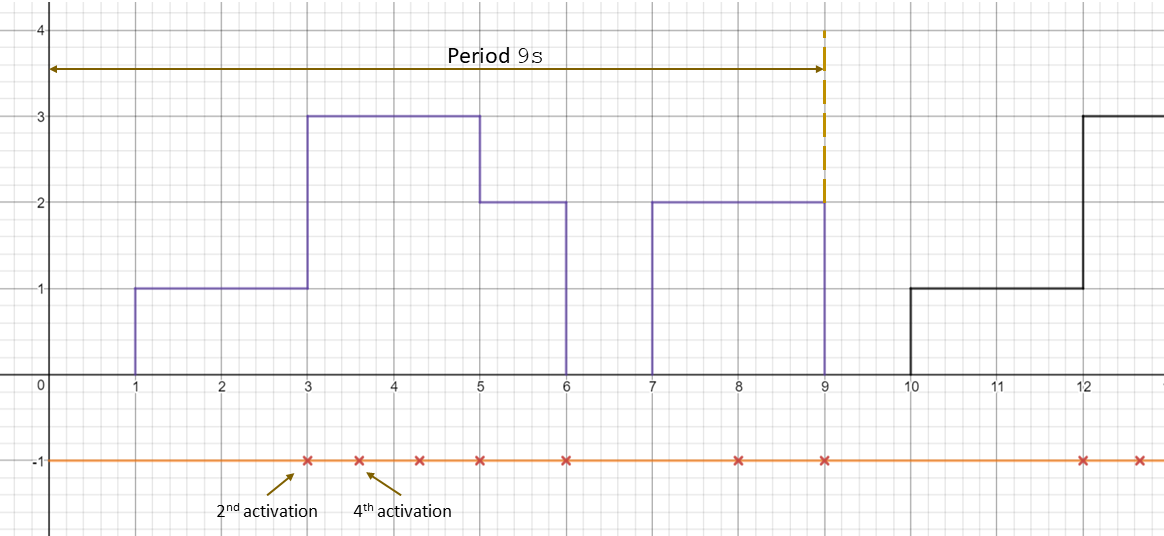
Example
The engine crankshaft is a good example in which Clocks can be used to model the behavior. Let's suppose a scenario in which a stimulus is triggered each time the rotating crankshaft reaches a specific angle.
In this example, the engine speed steeply increases from 3000rpm to 6000rpm in 5s, then the speed again decreases to 3000rpm in 5s. An stimulus shall be triggered when the engine crankshaft reaches 30 degrees. Triggering should repeat every two rotations.
Steeply increasing and decreasing pattern fits to the triangle clock function. The equations below show the calculations for the triangle clock function.
xOffset is added to make the triangle wave begin at the desired engine speed of 3000rpm:
-
yOffset = min.ticks = 3000rpm = 50rps = 50Hz
-
peakToPeak = max.ticks – min.ticks = 6000rpm – 3000rpm = 50Hz
-
period = 2 * risingSteepTime = 2 * 5s = 10s
-
xOffset = risingSteepTime / 2 = 2.5s
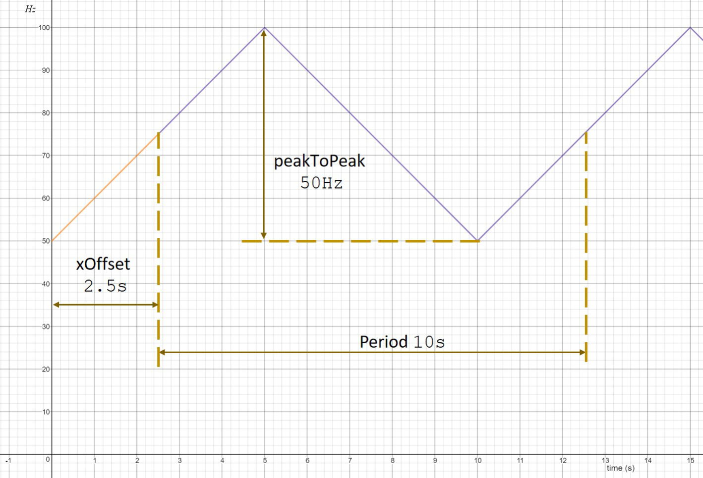
Task shall be triggered when the engine crankshaft reaches 30 degrees. Triggering should repeat for every two rotations. The scenario configuration for this example can then be derived as follows:
-
samplingOffset = firstTriggerAngle = 30
o / 360
o = 0.0833
-
samplingRecurrence = everySecondRotation = 2
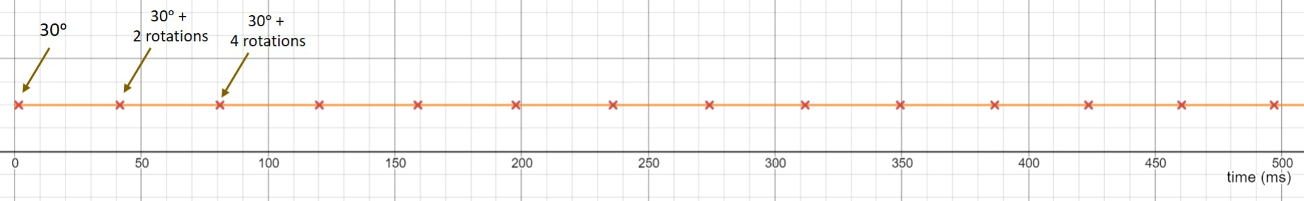
The engine crankshaft reaches 30 degrees at 1.66ms. From then on, the crankshaft completes 2 rotations at 41.49ms and 4 rotations at 81ms.
3.12.3 Mode Value List and Execution Condition
It is possible to change mode label values when a stimulus is executed. The mode labels and their new values are stored in the
set-mode-value-list. Via an
execution-condition modes also determine if a stimulus is executed.
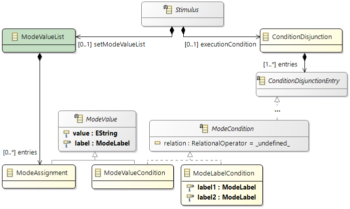
-
ModeValue: The
value string must be a valid element of the corresponding
Mode!
The
set-mode-value-list indicates: Each time the stimulus is executed all mode labels in this list are set to the corresponding value.
The
execution-condition is used to determine if a stimulus is executed.
3.13 Software Model
The AMALTHEA software model is central accessible through the
SWModel element.
3.13.1 Memory Information
Analyzing and mapping the software structure to available memories needs additional information of the included elements. This type of information targets the consumed size of memory of an element, represented by the
size attribute of type
DataUnit. The element
AbstractMemoryElement is a generalized element that provides this data. The following image shows the structure and also the elements of the software model that are extending
AbstractMemoryElement (the overview picture is only showing the hierarchy and not possible relationships between the elements):
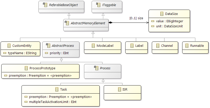
The label element represents a data element. It is directly located in a defined area of a given memory.
It can be used as a parameter, a temporarily existing variable or representing a constant value.
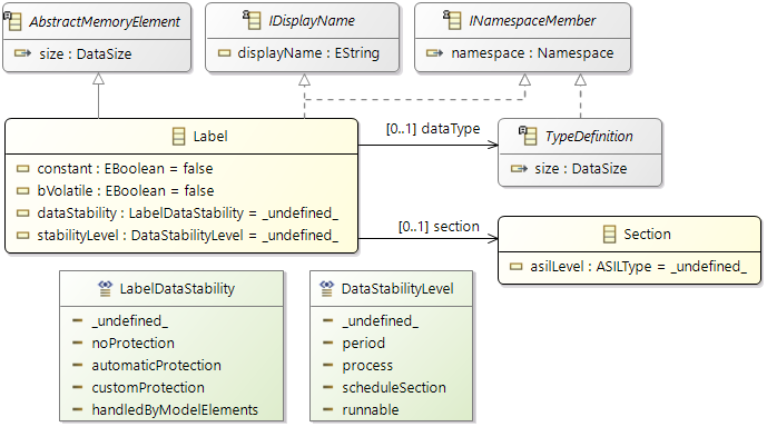
The following attributes are describing a label:
| Name |
Description |
|
name
|
The name represented as String value (derived from
AbstractElementMemoryInformation)
|
|
displayName
|
In addition to the name attribute, which must be unique, a label can also be described by an additional and optional display name. The displayName attribute must not be unique. It can be used for example to represent specification data, which can be different from the unique name (like a symbol) of an available software build. |
|
dataType
|
Reference to the data type definition |
|
constant
|
Boolean value to represent, if label is representing a constant value |
|
bVolatile
|
Boolean value to mark a label as volatile |
|
dataStability
|
Enumeration value to represent the data stability needs of the label. If set, it overwrites the global settings stated by the
OsDataConsistency, otherwise it inherits them (see OS Data Consistency).
|
|
stabilityLevel
|
Enumeration value to represent the data stability level of the label. If set, it overwrites the global settings stated by the
OsDataConsistency, otherwise it inherits them (see OS Data Stability).
|
The channel element has two different characteristics: it represents a data element in memory and also a way how runnables transmit larger amounts of data. A typical applications is the streaming of video data where a continuous sequence of images is sent in smaller chunks.
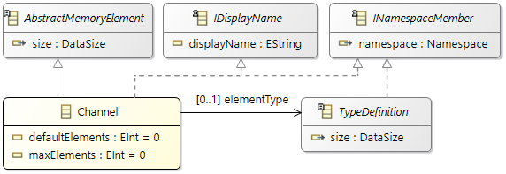
The following attributes are describing a label:
| Name |
Description |
|
name
|
The name represented as String value (derived from
AbstractElementMemoryInformation)
|
|
displayName
|
In addition to the name attribute, which must be unique, a label can also be described by an additional and optional display name. The displayName attribute must not be unique. It can be used for example to represent specification data, which can be different from the unique name (like a symbol) of an available software build. |
|
elementType
|
Reference to the data type definition of a single element |
|
defaultElements
|
Number of elements initially in the channel (at start-up) |
|
maxElements
|
Depth of channel (maximum number of elements that may be stored) |
General Information
The AMALTHEA data model supports meta information for data types. Therefore the element
TypeDefinition exists in the software part of the model. It consists of the name and size to define a data type.
BaseTypeDefinition has the additional possibility to define the representation of these data types in a target environment (e.g. AUTOSAR), represented by the
Alias element.
The compound data types are data structures, based on given or defined base types.
In the literature they are also often named composite or derived types
see Wiki.
The result of this type of definition is an own data type, which can be used as base data types.
They can consist of static structures or dynamic ones, like arrays or stacks.
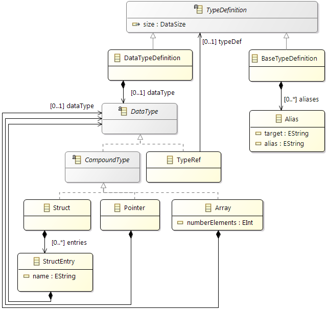
The following compound data type definitions are currently supported:
- Pointer: Holds a reference to another type using its memory address
- Array: Contains a number of elements of the same data type. The size of an array can be fixed or expandable.
- Struct: Contains other data types in a structured way, often called fields or members. The fields can be accessed by their name.
Sample
In the picture below a small sample is modeled containing the following information:
- Boolean type with size of 8 bits and alias for AR (Boolean) and C (bool)
- Char16 type with size of 16 bits and alias for AR (Char16) and C (short)
- charArray consists of 4 elements of type Char16
- "hello world struct" with the attribute name (charArray) and valid (Boolean)
Note: The picture shows the element types for better understanding!
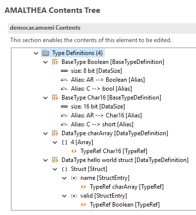
Activations are used to specify the intended activation behavior of
Runnables and
ProcessPrototypes. Typically they are defined before the creation of tasks (and the runnable to task mappings). So if there are no tasks defined, or if the mapping of runnables to tasks is not done, this is a way to document when the runnables should be executed.
Activations are independent of other top level elements in the AMALTHEA model. Single, periodic, sporadic, event or custom (free textual description only, no predefined semantic) activation pattern can be defined. This information can be used in the following development steps to create tasks, stimuli and the mappings to dedicated hardware.
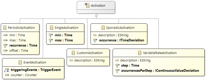
-
PeriodicActivation: The
Time object in the role of
min must not contain a negative value!
-
PeriodicActivation: The
Time object in the role of
max must not contain a negative value!
-
PeriodicActivation: The
Time object in the role of
offset must not contain a negative value!
-
PeriodicActivation: The
Time object in the role of
deadline must not contain a negative value!
-
SingleActivation: The
Time object in the role of
min must not contain a negative value!
-
SingleActivation: The
Time object in the role of
max must not contain a negative value!
The following figure shows the structure which describes
Tasks and Interrupt Service Routines (
ISR) in the AMALTHEA software model. The abstract class
Process generalizes ISRs and Tasks and provides the common attributes like the activation that is at runtime level represented by a
Stimulus. A
Task or
ISR contains
calls either to other Tasks (via inter process activation) or Runnables. These types of
calls are included in the
activityGraph attribute.
| Name |
Description |
|
name
|
Name of the process |
|
stimuli
|
Reference to one or more
Stimuli representing the different types of possible activations of this
Process
|
|
activityGraph
|
List of activities (e.g. runnable calls, label accesses). This specifies the behavior of the process. The objects will be executed in the same order they are stored in the list. |
|
preemption
|
Defines the preemption of a task by higher priority tasks. |
|
multipleTaskActivationLimit
|
Defines the maximum number of existing instances from the same task at any time, which is checked for load limitation reasons when a task is activated. If the multipleTaskActivationLimit is exeeded, the activation is ignored. See the "BTF Example" (User Guide > Examples) for an multipleTaskActivationLimit of 3. |
3.13.7 Runnables and Services
Both elements, runnables and services, are an abstraction of an executable entity. They are both represented by the
Runnable element and are distinguished by using the service attribute of type boolean.
Unlike tasks, which are activated in the context for the operating system, runnables are called by tasks or other runnables.
Runnables and Services in the AMALTHEA model can have call parameters. It is possible to specify the arguments of a service call and potential data dependencies. Based on these types of information, an additional analysis can be performed.
The next picture shows the general structure of the
Runnable element.
| Name |
Description |
|
callback
|
True if a runnable is used as a callback
|
|
service
|
True if
Runnable element can be seen in a service or global function manner. In more detail, the
Runnable is only called from other
Runnables and not directly from a
Task context.
|
|
activations
|
Although runnables in the simulation can only be called by tasks, it is possible to specify activation patterns for a runnable. |
|
executionCondition
|
It is possible to specify an execution condition for a runnable (depending on modes). |
|
activityGraph
|
Top level object containing
ActivityGraphItem objects, representing runtime, label accesses, other
Runnable accesses. The possibilities are described below.
|
|
tags
|
Can be used to annotate or group special kind of
Runnables
|
3.13.9 Activity Graph
A
ActivityGraph is the root container of
ActivityGraphItems. In addition some of the items can also contain sub items. These items are implementing the interface
IActivityGraphItemContainer.
The following picture shows the structure of a
Activity Graph. The
Activity Graph Items are used to define detailed behavior. With the
Switches it is possible to define alternative execution paths. The elements of the graph are executed in the order they are stored in the data model.
3.13.10 Activity Graph Items
The
ActivityGraphItems are describing the detailed behavior of a
Process or
Runnable. This can be either an abstraction of runtime or representing access to other elements like
Runnables,
Labels, and
Semaphores. An overview of the different possibilities is given in the next pictures.

Groups
A
Group is used to structure the
ActivityGraphItems.

| Name |
Description |
|
ordered
|
boolean attribute that indicates if the execution order of the contained elements is
fixed (default) or random.
|
|
interruptible
|
boolean attribute that specifies whether the group
can be interrupted (default).
If set to false the group cannot be interrupted (neither by interrupts nor by other higher priority tasks).
|
Some hints regarding
non-interruptible groups:
- they usually should be very short, so the system remains responsive
- they may not have nested groups among their contained items (this would result in a validation error)
- they should not be used for resource access synchronization across cores – there are Semaphores for that purpose
- they directly correspond to the sections between
SuspendAllInterrupts and
ResumeAllInterrupts calls in AUTOSAR
While Loop
A
WhileLoop enables to represent repetitions of activity graph items within an activity graph. These repeated items are contained in
items (from
ActivityGraphItemContainer). They will be repeated as long as the
condition is evaluated to be
true. In order to enter the while loop at all, the condition must initially be
true.

Switch
Switches can be used to define different execution paths within an activity graph. A
Switch corresponds to
if-else or
switch-case statements in a programming language. It uses the evaluated
ConditionDisjunction to decide which entry will be executed. The first fulfilled condition determines the path to execute.
A
SwitchEntry object is used to represent an execution path. A condition is defined for each entry (via
ConditionDisjunction).
At the
Switch it is also possible to define a default path, which is executed if none of the conditions of the
SwitchEntries is true.

Probability Switch
Each entry (path) of a
ProbabilitySwitch has a probability-value. As the name indicates, this is the value that defines the probability that the path is executed. It is computed as a fraction of its value divided by the sum of all
ProbabilitySwitchEntries in the surrounding switch.
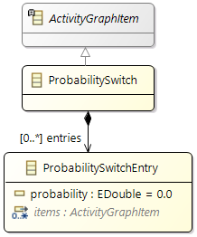
Ticks
Ticks allow to specify the required execution "time" in a basic way. They are the equivalent of cycles in the hardware domain and the execution time can easily be calculated if the frequency of the executing
ProcessingUnit (PU) is known.
Detailed definition: see Ticks
Execution Need
ExecutionNeed allows to specify the required execution "time" in a more abstract way. Multiple
NeedEntries can be used to specify execution characteristics. There is a map of default entries and (optional) maps of entries for specific hardware types (e.g. FPGA). These extended entries are also implemented as a map with a processing unit definition as the key.
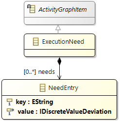
A simple approach (equivalent to the
RunnableInstructions in older versions of the AMALTHEA model) is the specification of the "number of generic instructions" that have to be executed. Together with the hardware feature "instructions per cycle (IPC)" and the frequency of a processing unit it permits the calculation of the execution time on a specific processing unit.
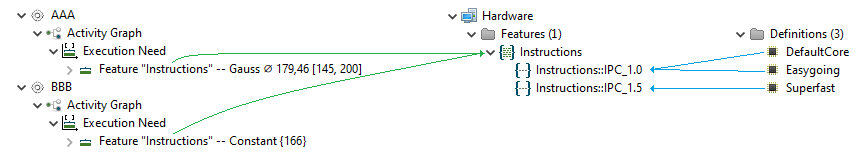
With the generic concept of
ExecutionNeeds it is also possible to describe more detailed characteristics, e.g. instruction mixes of floating point operations, integer operations, load/store operations, etc., or any other relevant aspect.
Calls and AUTOSAR communication
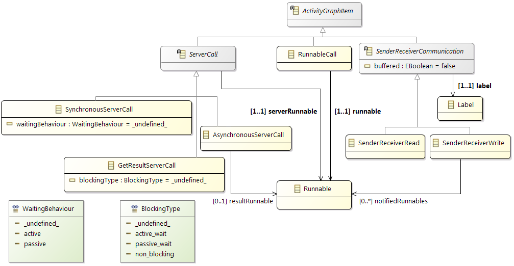
| Name |
Description |
|
RunnableCall
|
The activation of another
Runnable.
|
|
|
SenderReceiverCommunication
|
An abstract description for sender-receiver-communication (it can be read or write). |
|
ServerCall
|
An abstract description for client/server communication. It refers to a required runnable that describes the called server operation |
|
SynchronousServerCall
|
A synchronous server call with defined waiting behaviour. |
|
AsynchronousServerCall
|
An asynchronous server call with (optional) specification of result runnable. |
|
GetResultsServerCall
|
Get the result of a previous asynchronous server call (with defined blocking behaviour). |
Label Access
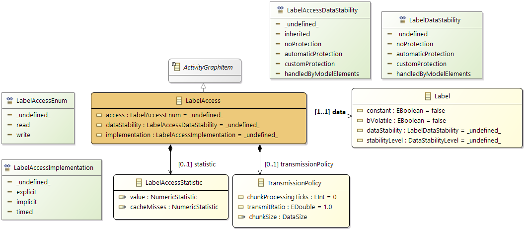
| Name |
Description |
|
access
|
The type of access is represented using the values of
LabelAccessEnum.
|
|
data
|
Describes the access to an existent
Label (set as reference).
|
|
dataStability
|
Describes the data stability needs. If set, it overwrites the label settings, otherwise it inherits them (see OS Data Consistency). |
|
implementation
|
Describes how a label access is implemented: -
explicit: also known as "direct"
-
implicit: also known as "optimized"
-
timed
|
|
statistic
|
Defines the frequency of the label access. |
|
transmissionPolicy
|
The following attributes reflect the computing demand (time) depending on data: -
chunkSize: Size of a part of an element, maximum is the element size.
-
chunkProcessingTicks: Number of ticks that will be executed to process one chunk (algorithmic overhead).
The next attribute specifies the amount of data actually accessed by a runnable (required to analyze memory bandwidth demands): -
transmitRatio: Specify the ratio of each element that is actually transmitted by the runnable in percent. Value must be between [0, 1], default value is 1.0 .
|
Channel Access
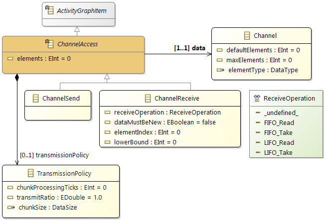
Common attributes:
| Name |
Description |
|
data
|
Describes the access (
ChannelSend or
ChannelReceive) to an existent
Channel (set as reference).
|
|
elements
|
Maximum number of elements that are transmitted. |
|
transmissionPolicy
|
The following attributes reflect computing demand (time) depending on data: -
chunkSize: Size of a part of an element, maximum is the element size.
-
chunkProcessingTicks: Number of ticks that will be executed to process one chunk (algorithmic overhead).
The next attribute specifies the amount of data actually accessed by a runnable (required to analyze memory bandwidth demands): -
transmitRatio: Specify the ratio of each element that is actually transmitted by the runnable in percent. Value must be between [0, 1], default value is 1.0 .
|
Receive attributes:
| Name |
Description |
|
receiveOperation
|
The type of an operation is defined by LIFO or FIFO, Read or Take: -
LIFO: last-in, first-out
-
FIFO: first-in, first-out
-
Read: reads elements (without modifying the channel content)
-
Take: removes the received elements
|
|
elementIndex
|
Position (index) in channel at which the operation is effective. Zero is the default and denotes the oldest (FIFO) or newest element (LIFO) in the channel. |
|
lowerBound
|
Minimum number of elements returned by the operation. The value must be in the range [0,n], with n is the maximum number of elements that are received. Default value is n. |
|
dataMustBeNew
|
Specify if the operation must only return elements that are not previously read by the runnable. Default value is false. |
Semaphore Access

| Name |
Description |
|
SemaphoreAccess
|
Represents an access of a Semaphore. The type of access is defined using the
SemaphoreAccessEnum values. The
Semaphore itself is set as a reference to an existent one.
|
|
access
|
Defines the type of access (request, exclusive, release). Note that for spinlocks and mutexes, a request access is always exclusive, so
request means the same as
exclusive in these cases.
|
|
waitingBehaviour
|
Defines if the process is blocking the core when it waits (active) or not (passive). Note that for spinlock accesses, only active waiting can be used. |
-
SemaphoreAccess: The
waitingBehaviour can only be
active if the accessed semaphore is a spinlock!
Mode Label Access
| Name |
Description |
|
ModeLabelAccess
|
Describes the access to an existing
ModeLabel (set as reference). The type of access is represented using the values of
ModeLabelAccessEnum: -
read: indicates that the behavior of the runnable is influenced by the current value of the
ModeLabel.
-
set: represents the change of a mode label. The defined
value is set.
-
increment /
decrement: changes a mode label. The value is increased / decreased by
step. In case of an
EnumMode the next / previous literal is set (according to
step limited by the range of literals).
|
-
ModeLabelAccess: The
value string must be a valid element of the corresponding
Mode!
Custom Event Trigger
The
Custom Event Trigger references an event of type
Custom Event. The execution of a
Custom Event Trigger entry triggers the corresponding event that can be observed by an
Event Stimulus.
Enforced Migration
Each task is controlled by at least one task scheduler. A task scheduler is the resource owner of one or multiple processor cores (The task scheduler decides on which of its cores the task is executed). The
Enforced Migration forces the task to switch to another task scheduler. Therefore the
Enforced Migration entry contains a reference to the new task scheduler.
This element is used as a short notation to simplify the simulation of different design possibilities. It should normally be modeled as two separate tasks and an inter process trigger.
Inter Process Trigger
The
Inter Process Trigger references a stimulus of type
Inter Process Stimulus. The execution of an
Inter Process Trigger entry triggers the processes that are mapped to this stimulus.
Schedule Point
At a
Schedule Point, the process calls the scheduler that currently administrates it. This is used for cooperative task scheduling (see OSEK Specification 2.2.3, 2005).
Terminate Process
If a
Terminate Process is reached during the execution of a
Activity Graph, the
Task or
ISR terminates immediately. It is not required to insert this element at the end of a
Activity Graph. It can be used to define an execution path (by using
Switches) that terminates a process.
Wait/Clear/Set Event
The AMALTHEA Software Model contains a list of
OS-Event objects. These can be used for task synchronization. Elements are
Wait Event,
Clear Event and
Set Event.
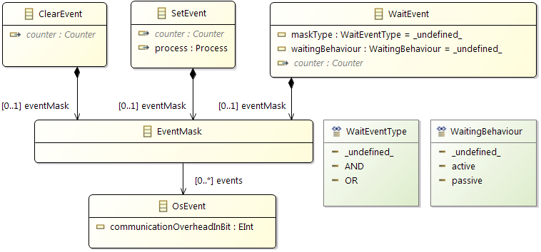
With
Wait Event the process waits for a number of events (defined in the
Event Mask) to be set. Here it can be defined if the process waits just for one of the
OS-Events (maskType = OR) or for all of them (maskType = AND). The
waiting behaviour defines if the process is blocking the core when it waits (active) or not (passive).
Set Event sets/fires a list of
OS-Events. Here it is possible to define a context for the
OS-Event. If a process is referenced, then the
OS-Events are set just for this process.
The execution of a
Clear Event entry unsets all referenced
OS-Events.
For more information about OS-Events, see the OSEK Specification 2.2.3, 2005.
Statistical Values
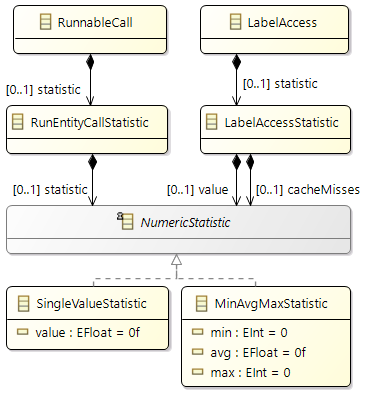
It is possible to add to different elements (as shown in the picture above) different types of statistical values. These values can be used to describe in more detail the following behaviors:
-
RunEntityCallStatistic: Can be used to describe in more detail the dynamic call behavior of a
RunnableCall. The value is representing how often the call is performed.
-
LabelAccessStatistic: Describes in more detail the dynamic behavior accessing a
Label by having cache misses or how often a read/write is performed.
The next diagram shows the overall picture, the sub chapters describe the details.
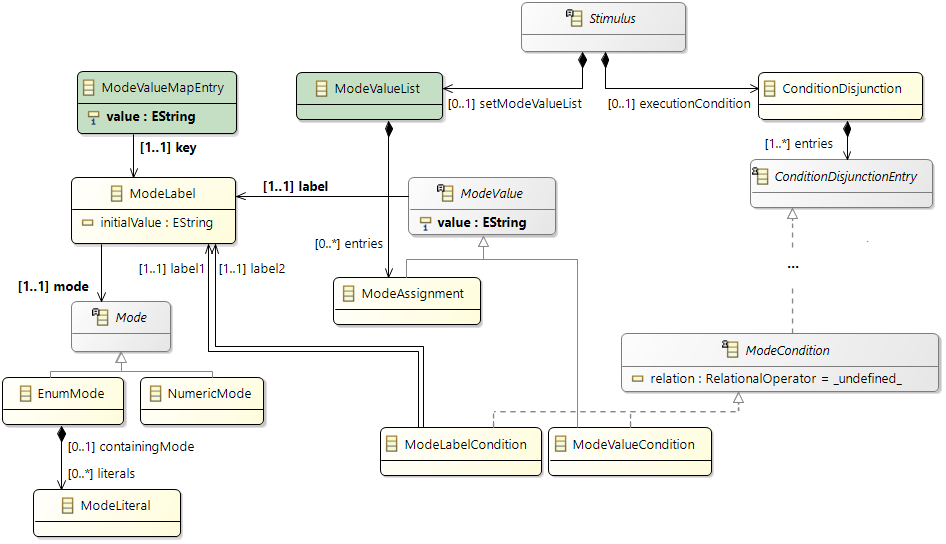
The actual state of a Mode is represented by a
ModeLabel or a
LocalModeLabel.
The (global) mode labels are mainly used in
Mode Conditions to describe the conditional execution of a
Runnable or a
Stimulus.
Local mode labels are defined in the context of an executable and can be modified in the activity graph.
Both types of mode labels can be used to determine which path should be executed in a
Switch statement or how often the body of a
WhileLoop should be repeated.
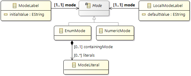
The
Mode element denotes the type and the possible values of a specific system state. The subclasses
EnumMode and
NumericMode describe the values that are allowed for the corresponding
ModeLabel. In case of a
EnumMode the
initialValue has to be the name of one of the contained
ModeLiterals. For
NumericMode the
initialValue has to be the string representation of an integer.
Both
Mode Label elements are a concrete representation of a specific
Mode. They are described using the following attributes:
| Name |
Description |
|
name
|
Name of the mode label |
|
displayName
|
In addition to the name attribute, which must be unique, a mode label can also be described by an additional and optional display name. The displayName attribute must not be unique. It can be used for example to represent specification data, which can be different from the unique name (like a symbol) of an available software build. |
|
mode
|
Reference to the corresponding
Mode definition
|
|
initialValue
|
String representation of the initial value (of a mode label) |
|
defaultValue
|
String representation of the default value (of a local mode label) |
Mode Changes
The value of a (global) mode label can be changed using the set-mode-value-list of a
Stimulus.
Another possibility is a write access within an
Activity Graph via a
Mode Label Access or
Local Mode Label Assignment.
Mode Conditions
Mode conditions allow to specify dedicated states of the overall system.
Depending on the condition evaluation switches can be executed or stimuli can be influenced.
The ModeValueMap represents the system state that has to be provided as an external input, e.g. from a simulation or analysis tool.

3.13.13 Local Mode Labels
Local mode labels are defined in the context of an executable (Task, ISR or Runnable).
The class diagram shows the abstract class
LocalModeValue that provides the connection between a local mode label and a value source.
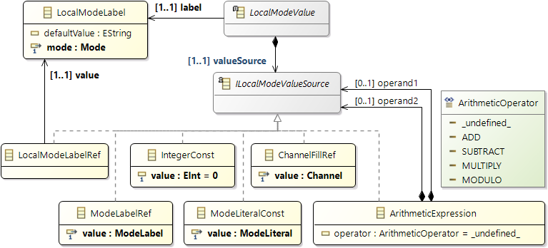
Possible value sources:
- Constants (integer values or mode literals)
- Values of other mode labels
- Fill levels of channels
- Arithmetic expressions
The subclasses are used for comparison and assignment.
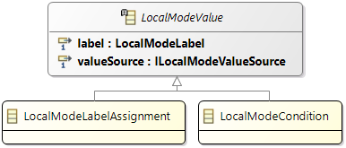
Local Mode Label Assignment
The
Local Mode Label Assignment offers a number of possibilities to change the value of a local mode label. Values can be constant, the copied value of another mode label or even the result of an arithmetic expression.
The
Mode Label Assignment simply provides a way to copy the content of a local mode label to a global one.
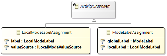
Local Mode Conditions
Local mode conditions are available where local mode labels are accessible. That means they can be used in
Switch or
WhileLoop statements in the activity graph of an executable.
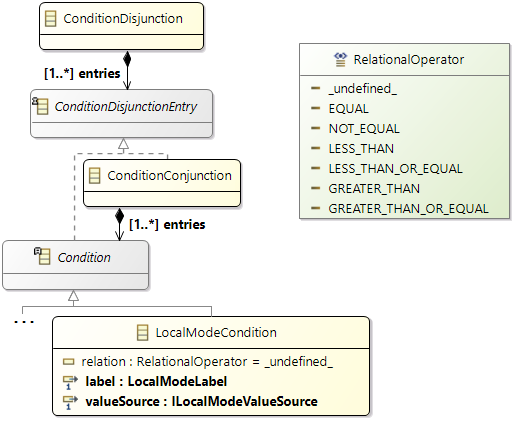
Local mode label examples
The following example shows a local mode label "loop1" that represents a numeric mode called "Counter". It is defined in the scope of the runnable "ABSCalculation". This scope is also seen in all references to the local mode label where the qualified name "ABSCalculation.loop1" has to be used. The value of the local mode label is modified and checked by several items of the activity graph: the value is set, checked in the loop condition of a while loop and decremented in the loop body. The last line shows that it is also possible to store the value of a local mode label in a (global) mode label.
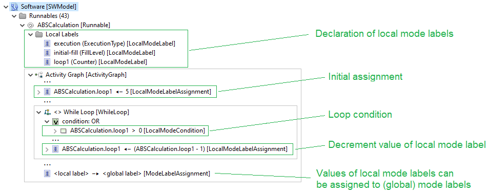
The local mode labels of an executable are available only during the execution. The next part of the example shows how to initialize local mode labels of the called runnable as part of the runnable call. This feature allows to set the context of a specific invocation and the runnable can react accordingly (e.g. by executing different paths of the activity graph).
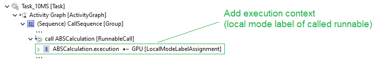
3.13.14 Process Prototypes
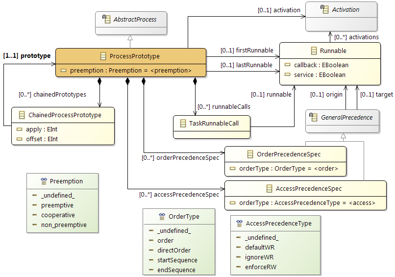
In addition to the Task elements, the AMALTHEA model contains an element process prototype.
This prototype can be used to define raw data of a task. It can be used to specify access to
labels (read, write) or other runnables/functions as possible with the normal task, but not the
order of the access. These prototypes are then processed by different algorithms. The algorithms are creating the tasks, are filling, verifying or modifying the data based on their different checks. The final result of this processing are tasks, which are corresponding to the data of the prototypes.
These tasks are representing the current state and can be further processed, for example to generate code or further simulation. With the process prototypes available in the model, it is possible to define the structure of the software in an early development phase. The implementation at that moment is open and not yet completed, but the general idea can be verified.
Another issue can be the distribution to a multi-core system, coming from a single-core system. Therefore the activity graph can be analyzed and computed to get the right order and parallelization of the elements and dependencies.
3.13.15 Process Chains
The following figure shows the structure which describes
Process Chains in the AMALTHEA software model. A process chain is used to group task and isrs together which are executing after each other and represent an end-to-end data processing path. The processes inside a process chain are connected via
Inter Process Activations.
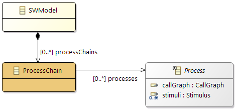
The following attributes are describing a process chain:
| Name |
Description |
|
name
|
Name of the process chain |
|
processes
|
List of tasks and isrs which are included in the process chain |
3.13.16 Custom Entities
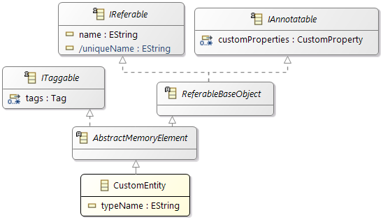
The
CustomEntity element defines a way to add not yet available elements of the software model in a generic way. The only contained attribute defines the type of the entity by setting it as a
String. Additional properties can be set using the
CustomAttributes.
Section (Virtual Memory Section) is used to group the memory elements (Labels, Runnables). This is achieved by associating the
Section element to
Label &
Runnable elements
Below are properties of Section element:
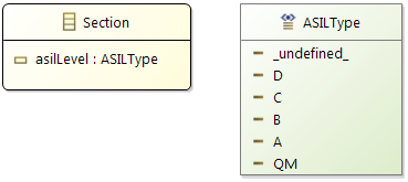
With this type of information available, the complexity of mapping software components to memories can be reduced. The next picture gives an overview about the general idea of the mapping with Sections.
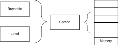
3.13.18 Data Dependencies and Runnable Parameters
Overview
The purpose of following model elements is to describe a high level data flow. Parameters of runnables (or services) and specific call arguments allow to model a behavior that depends on the call tree but the detailed computation and the control flow within a runnable are not taken into account. Therefore only "potential" influences are modeled. The following picture shows this data flow with dashed lines.
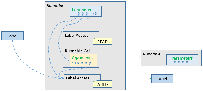
Elements with data dependency
The data flow is specified with "depends on" references. Elements that can specify a dependency are:
-
LabelAccess
of type "WRITE"
-
CallArgument
that refers to an "IN" (or "INOUT") parameter
-
RunnableParameter
with direction "OUT" (or "INOUT")
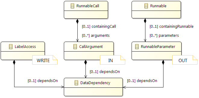
Data Dependency
A data dependency defines the elements that can influence a value that is written or transferred. Possible origins are:
-
Label
-
RunnableParameter
with direction "IN" (or "INOUT")
-
CallArgument
that refers to an "OUT" (or "INOUT") parameter
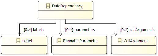
4 Developer Guide
4.1 Overview of Features and Plug-ins
There are two top-level features of the AMALTHEA Tool Platform, the AMALTHEA Tool Platform and the AMALTHEA Tool Platform SDK features. The non-SDK feature contains everything you need to run the AMALTHEA tools and models. If you like to develop new tools on top of the models or extend the models you may need the SDK. It contains beside the runtime all sources.
The top-level feature itself contains basic platform plug-ins and tools as well as several sub-features. These are
- APP4MC Platform – Platform (includes all features and 3rd party libraries).
- APP4MC Docu – Basic Help (is extended by loading other features).
- APP4MC Examples – Examples that can be added by the example wizard.
- AMALTHEA Models – AMALTHEA models (EMF) and utility functions.
- AMALTHEA Edit – AMALTHEA model edit support.
- AMALTHEA Editors – Editors for the models.
- APP4MC Validation – Model validations (can be selected and executed on demand).
- AMALTHEA Visualizations – Model visualizations (show additional info on selected model element).
- AMALTHEA Converters – Independent feature for AMALTHEA model migration.
- AMALTHEA Workflow Common – Basic elements to define workflows on the model.
- AMALTHEA Workflow – Defining workflows (based on MWE2 workflow engine).
- AMALTHEA Workflow Scripting – Defining workflows (based on EASE scripting).
- APP4MC Tracing – Record, analyze and transform runtime traces of the embedded system.
- AMALTHEA Import – Import of the models.
- AMALTHEA Export – Exports of the models.
For all features there also exists an SDK containing the sources. If you install the AMALTHEA Tool Platform SDK, it contains all features as SDKs.
The plug-ins are organized in various namespaces. The ids of most plug-ins containing models are within the namespace
org.eclipse.app4mc.amalthea.model, whereas examples can be found in plug-ins named
app4mc.example.
4.2 Model Visualization
4.2.1 Visualization framework
The plug-in
org.eclipse.app4mc.visualization.ui provides a small framework to visualize model elements. It contains a view part
VisualizationPart that can be opened via
-
Window → Show View → Other... → APP4MC → APP4MC Visualizations,
- or via right click on an element and selecting
Open APP4MC Visualization.
Via the context menu it is also possible to open multiple instances of the
VisualizationPart.
On selecting a model element, the VisualizationPart is updated to render a corresponding visualization. The visualization to render is searched in the ModelVisualizationRegistry OSGi service. If multiple visualizations are registered, the first one will be selected by default, unless the user has selected another visualization before.
The visualization view has 4 entries in the toolbar:
-
Visualization dropdown
The dropdown contains all available visualizations for the current active selection. A click on the image will reload the visualization.
-
Pin visualization
The selection handling will be disabled so the visualization gets not updated on model selection changes.
-
Select model element
Selects the current visualized model element in the model editor. Useful for example if a visualization is pinned and the selection in the model editor changed.
-
View Menu
Contains entries to customize title and supported visualizations of the current view.
The whole red area can be used to render the visualization.
4.2.2 Contributing a new model visualization
To contribute a new visualization to the framework, the followings steps have to be done:
- Create a new plug-in for the visualization contribution.
- Add at least the following dependencies:
- Required Plug-ins
-
org.eclipse.jface
(to be able to contribute to the view)
- Imported Packages
-
org.eclipse.app4mc.amalthea.model
(to get access to the model element that should be rendered)
-
org.eclipse.app4mc.visualization.ui.registry
(needed to import the necessary interface)
-
org.osgi.service.component.annotations: In the properties, select Minimum Version as
1.3.0 inclusive
(needed to get access to the OSGi DS annotations)
- Create a new Visualization implementation that follows this pattern:
@Component(property= {
		"name=Runnable Visualization",
		"description=Render the name of the Runnable"
})
public class SampleVisualization implements Visualization {

	@PostConstruct
	public void createVisualization(Runnable runnable, Composite parent) {
		Label label = new Label(parent, SWT.NONE);
		label.setText(runnable.getName());
	}
}
To register the Visualization implementation the framework utilizes OSGi DS. This means:
- The class needs to implement
Visualization (only a marker interface needed for OSGi service injection)
It is mandatory to place this class inside a user defined package (i.e., other than default package)
- The class needs to be annotated with
@Component (ensure DS annotation support is enabled in your workspace)
To enable DS annotation for the entire workspace,enable the following option in your eclipse workspace at:
Window -> Preferences -> Plug-in Development -> DS Annotations -> "Enable descriptors from annotated sources"
Once above steps are followed, visualization plugin contents should look like below:
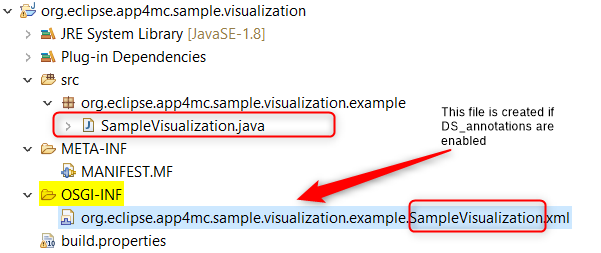
The Visualization will automatically be registered in the
ModelVisualizationRegistry with the appropriate meta-data. The meta-data is extracted from the class definition and the method annotated with
@PostConstruct. Additionally information can be provided via component properties on the
@Component annotation.
The following component properties are supported:
- id
- Defaults to the fully qualified class name of the service.
Used to uniquely identify the last selected visualization.
- name
- Defaults to the simple class name of the service.
Used in the visualization dropdown as label of the menu item.
- description
- Defaults to null.
Used in the visualization dropdown as tooltip of the menu item.
- type
- Defaults to the type of the first parameter of the @PostConstruct method.
Used to register the visualizations for a given model type.
Note: It is not recommended to override the type configuration.
The rendering is triggered via Eclipse injection mechanisms. Therefore a method annotated with
@PostConstruct needs to be created. This method needs at least two parameters in the following order:
-
Model type or
java.util.List<Model type>
The first parameter needs to be the type or a List of the type that should be handled by this Visualization.
-
Composite
The parent Composite on which the rendering should be performed.
So the following method signatures would be valid for Visualizations for Runnable model elements:
@PostConstruct
public void createVisualization(Runnable runnable, Composite parent) {}

@PostConstruct
public void createVisualization(List<Runnable> runnable, Composite parent) {}
You can specify additional parameters that should be injected. Only the first parameter has a semantic to be able to extract the model type for which the Visualization is implemented.
Additionally a method annotated with
@PreDestroy can be added that gets called before the Visualization is disposed. This gives the opportunity to clean up resources if necessary.
As the service instance creation is done by the OSGi Service Component Runtime, the following information needs to be considered with regards to injection:
- You can use @Reference to get other OSGi services injected.
- There is no field or constructor injection available via Eclipse injection.
(usage of @Inject on fields or constructors will not work)
- In general you should not use fields/members to store rendering related information on an instance level.
4.3 Model Validation
4.3.1 Validation framework
APP4MC contains a flexible framework based on standard EMF validations.
The main plugins:
- org.eclipse.app4mc.validation.core
- Basic interfaces and helper classes to organize and execute validations.
- org.eclipse.app4mc.validation.ui
- User interface components: profile selection dialog, marker helper.
- org.eclipse.app4mc.amalthea.validations
- AMALTHEA standard profile and validations
4.3.2 Validations
Validations have to implement the IValidation interface. Additional information is specified with annotations:
Example:
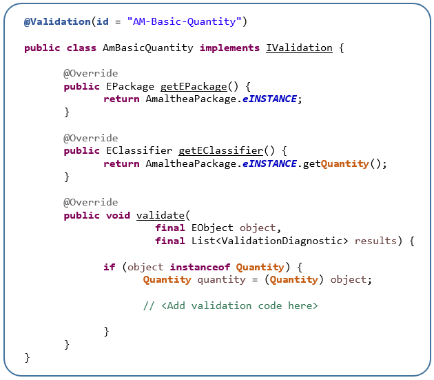
Profiles have to implement the IProfile interface. Details are specified with the following annotations:
- @Profile
- @ProfileGroup
- @ValidationGroup
Example:
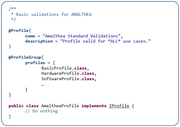
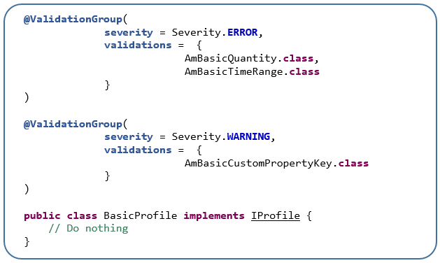
4.4 Model Workflow
4.4.1 Introduction
The APP4MC AMALTHEA platform provides the option to define a workflow on a model with different steps. AMALTHEA provides a simple API for implementing such a workflow. The definition of the workflow can be done either in plain Java or any other language, which is able to access Java classes.
The
EASE framework provides a scripting environment inside of Eclipse with different script engines like Rhino (JavaScript), Jython or Groovy. AMALTHEA provides a sample and some convenient helpers based on EASE to define and execute such a workflow.
As an alternative APP4MC provides also an implementation for the
Modeling Workflow Engine 2 (MWE2), coming from the Xtext framework. The definition of the workflow can be done in a textual syntax from MWE2, containing different components which are working on the given model.
AMALTHEA provides several plugins for this purpose:
- org.eclipse.app4mc.amalthea.workflow.core
- Includes basic API and some predefined workflow components, which can be used independent from any framework.
- org.eclipse.app4mc.amalthea.workflow.ease
- Provides some helper modules for EASE
- org.eclipse.app4mc.amalthea.workflow.mwe2
- Provides basic classes for usage with MWE2
4.4.2 General Structure
The plugin
org.eclipse.app4mc.amalthea.workflow.core provides a general abstract class
org.eclipse.app4mc.amalthea.workflow.core.WorkflowComponent which can be used to extend in the case to provide or implement an own workflow step.
It provides the following features:
- Defines the constant
AMALTHEA_SLOT, which can be used to store and retrieve the AMALTHEA model from the
org.eclipse.app4mc.amalthea.workflow.core.Context.
- Provides some convenient methods to retrieve the model from the context, get a copy of the model or store the model in the context.
The interface
org.eclipse.app4mc.amalthea.workflow.core.Context provides convenient methods to store and retrieve data in a
org.eclipse.app4mc.amalthea.workflow.core.WorkflowComponent.

The class
org.eclipse.app4mc.amalthea.workflow.core.DefaultContext is a default implementation using an internal
java.util.HashMap to store the data.
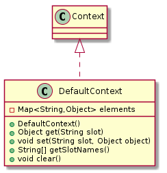
A sample workflow implementation with two components
WorkfklowComponent1 and
WorkflowComponent2 can look like the following structure.
Both classes are extending
org.eclipse.app4mc.amalthea.workflow.core.WorkflowComponent.
The next step is to create a
WorkflowDefinition, which needs to do the following steps:
- Create an instance of a
org.eclipse.app4mc.amalthea.workflow.core.Context using the
org.eclipse.app4mc.amalthea.workflow.core.DefaultContext
- Create an instance of
WorkflowComponent1 and configure it if needed with the proper setter methods
- Call the
run method of
WorkflowComponent1 and pass the context
- Create an instance of
WorkflowComponent2 and configure it if needed with the proper setter methods
- Call the
run method of
WorkflowComponent2 and pass the context
Therefore using the context, data can be shared between the different workflow component implementations.
The following diagram is showing this flow in more detail:
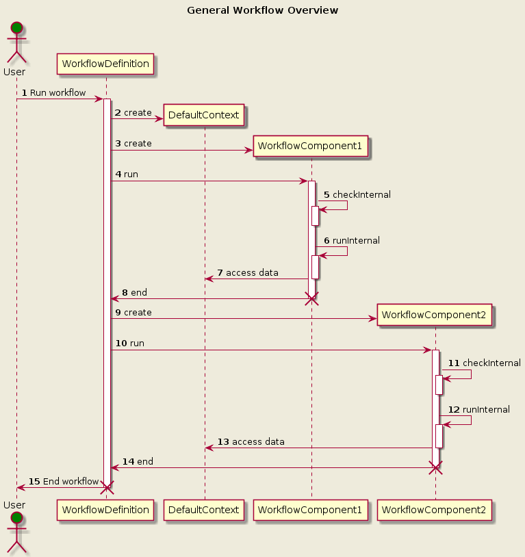
4.4.3 Available Basic Components
The APP4MC AMALTHEA platform ships with some available workflow steps, which can be used out of the box.
Model Reader
The component
org.eclipse.app4mc.amalthea.workflow.component.ModelReader reads a given list of files containing AMALTHEA models. The result model is stored in the
AMALTHEA_SLOT as default. Please refer the JavaDoc for more details.
Simple configuration inside of a workflow can look like the following:
ModelReader reader = new ModelReader();
reader.addFileName("path to file");
reader.run(ctx);
Model Writer
The component
org.eclipse.app4mc.amalthea.workflow.component.ModelWriter writes a given AMALTHEA model to either one file or several files. As default the current available model in the
AMALTHEA_SLOT is taken.
The following parameters are available to set:
-
boolean singleFile default
true
-
String
outputDir
-
String
fileName, if output is set to split files the different models are separated by an additional suffix in the name indicating the contained model.
Sample configuration inside of a workflow:
ModelWriter writer = new ModelWriter();
writer.setOutputDir("path to dir");
writer.setFileName("output.amxmi");
writer.run(ctx);
Add Schedule Points
The component
org.eclipse.app4mc.amalthea.workflow.component.AddSchedulePoints modifies a given model (default in the
AMALTHEA_SLOT) in that way, that in the
org.eclipse.app4mc.amalthea.model.sw.SWModel the contained
org.eclipse.app4mc.amalthea.model.sw.Task elements are checked if the preemption is set to cooperative. If this is the case, it will add between the elements of the
org.eclipse.app4mc.amalthea.model.sw.CallGraph new elements of type
org.eclipse.app4mc.amalthea.model.sw.SchedulePoint.
Sample configuration inside of a workflow:
AddSchedulePoints addSchedulePoints = new AddSchedulePoints();
addSchedulePoints.run(ctx);
4.4.4 EASE modules
The purpose of using EASE is to provide one way to define and run a workflow for a model.
Therefore APP4MC provides some helper methods to be used in the
EASE scripting environment.
The modules are provided by the plugin
org.eclipse.app4mc.amalthea.workflow.
ease
.
Workflow Module
The workflow module provides some helpers regarding running a APP4MC workflow definition based on EASE.
The general module can be loaded with the following line:
loadModule('/APP4MC/Workflow')
EASE opens an own Eclipse console by default to show the output of the executed script when using right click and
Run as -> EASE Script. Therefore if you are using Log4J for your logging, you can use the following provided methods to configure dedicated Log4J Loggers to use also the EASE console for output.
The following overview gives an overview about the available helper methods:
| Method |
Params |
Description |
| addLoggerToConsole |
String loggerName |
Adds a Log4J logger to the output of the current used output of the EASE script engine. |
| addLoggerToConsole |
String loggerName, String pattern |
Adds a Log4J logger to the output of the current used output of the EASE script engine with a given pattern, see
org.apache.log4j.PatternLayout for more details
|
| endWorkflow |
- |
Basic finish actions to be performed, should be called at the end |
4.4.5 MWE2 Workflow
The plugin
org.eclipse.app4mc.amalthea.workflow.
mwe2
provides a general class
org.eclipse.app4mc.amalthea.workflow.base.AmaltheaWorkflow which can be used to extend in the case to provide or implement an own workflow step based on
Modeling Workflow Engine 2 (MWE2).
It provides the following features:
- Extends
org.eclipse.emf.mwe.core.lib.WorkflowComponentWithModelSlot
- Defines the constant AMALTHEA_SLOT, which can be used to store and retrieve the AMALTHEA model from the
org.eclipse.emf.mwe.core.WorkflowContext.
- Provides some convenient methods to retrieve the model from the context, get a copy of the model or store the model in the context.
To use the AMALTHEA model workflow component, currently the following dependencies are needed in addition to the AMALTHEA model plugins:
- org.eclipse.app4mc.amalthea.workflow.mwe2
- org.eclipse.emf.mwe2.lib
- org.eclipse.emf.mwe2.launch
- org.apache.log4j
MWE2 Components
The APP4MC AMALTHEA platform ships with some available workflow steps for usage together with MWE2.
Note: To use the components below as shown in the corresponding configurations, the classes must be imported!
Reader
The component
org.eclipse.app4mc.amalthea.workflow.mwe2.util.AmaltheaReader reads a given list of files containing AMALTHEA models. The result model is stored in the
AMALTHEA_SLOT as default.
Sample configuration inside of a workflow:
component = AmaltheaReader {
	fileName = "${base}/model/AMALTHEA_Democar_MappingExample.amxmi"
	fileName = "${base}/model/AMALTHEA_Democar_MappingExample-hw.amxmi"
}
Writer
The component
org.eclipse.app4mc.amalthea.workflow.mwe2.util.AmaltheaWriter writes a given AMALTHEA model to either one file or several files. As default the current available model in the
AMALTHEA_SLOT is taken.
The following parameters are available to set:
- boolean singleFile default true
- String outputDir
- String fileName, if output is set to split files the different models are separated by an additional suffix in the name indicating the contained model.
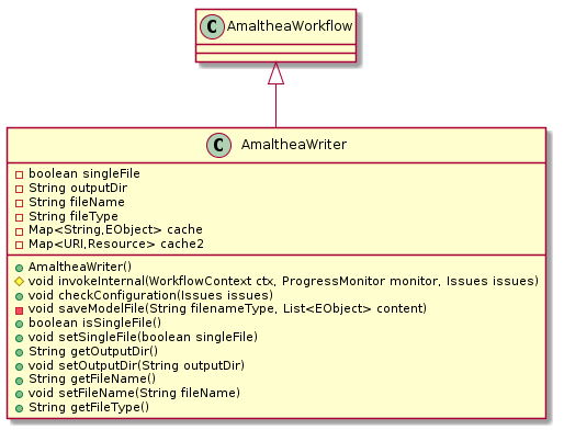
Sample configuration inside of a workflow:
component = AmaltheaWriter {
	fileName = "createtasks"
	singleFile = true
	outputDir = "${base}/workflow-output"
}
Add Schedule Points
The component
org.eclipse.app4mc.amalthea.workflow.mwe2.util.AddSchedulePoints modifies a given model (default in the AMALTHEA_SLOT) in that way, that in the
org.eclipse.app4mc.amalthea.model.SWModel the contained
org.eclipse.app4mc.amalthea.model.Task elements are checked if the preemption is set to cooperative. If this is the case, it will add between the elements of the
org.eclipse.app4mc.amalthea.model.CallGraph new elements of type
org.eclipse.app4mc.amalthea.model.SchedulePoint.
Sample configuration inside of a workflow:
component = AddSchedulePoints {
}
4.4.6 Current Limitations / Open Points
As there are two options available (Basic Java/EASE and MWE2 based) for running a workflow, there are currently also some limitations existent. The following table should help you to chose the right base:
| Use Case |
Supported in MWE2 |
Supported in EASE |
Reason |
| Loading of AMALTHEA model files (with cross document references) using workflow/script file |
no
|
yes
|
-
MWE2: Separate Java runtime is started by MWE2, Sphinx relies in running Eclipse instance
-
EASE: Makes use of the runtime from runtime workbench
|
| Using workflow components which are available in the runtime (i.e. workflow component classes which are already available in plugins as a part of the runtime product) |
yes
|
yes
|
-
MWE2: Separate runtime is started by MWE2 and if plugin (containing workflow component) is added as dependency then its classes are loaded
-
EASE: Makes use of the runtime from runtime workbench and has access to all classes
|
| Defining custom workflow components (Java classes) and using them in the workflow/script file located in the same workspace |
yes
|
yes
|
-
MWE2: Custom workflow component objects can be directly created in MWE2 script file(as in Java) and there is no restriction [irrespective of whether there is constructor]
-
EASE: As the runtime from the launched workbench (runtime workbench) is used, custom Java classes available in the workspace are not part of the classpath. For creation of objects of custom workflow components (Java classes): EASE JVM module
createInstance API should be used by specifying the absolute path of the Java class
|
| Using Java classes (available in the runtime workspace from other plugins --> these classes are not part of runtime workbench) inside custom workflow component Java classes |
yes
|
yes
|
-
MWE2: works perfectly (just like native)
-
EASE: works, for creation of object from custom Java classes, EASE JVM module is used, which compiles the used Java classes and creates objects of them
|
| Using classes (API) from 3rd party libraries (added in the classpath of the plugin)inside custom workflow component java classes |
yes
|
yes(*)
|
-
MWE2: As new Java runtime is created, all the required plugins & jars are added in the classpath
-
EASE: The runtime from workbench and the jars from the classpath of a plugin (created newly in the runtime workbench) are loaded by EASE.
|
*: This feature is only available for EASE versions newer than 0.3.0. Older versions will fail with an exception java.lang.NoClassDefFoundError: <your used class from 3rd party lib>
Sample for using EASE JVM module to load a class from the same workspace:
var labelsCreationComponent = createInstance("workspace://com.ease.example/src/org/eclipse/app4mc/amalthea/example/workflow/components/CreateLabelsComponent.java")
4.4.7 Adding a new workflow component
Below you will find a sample how to add and implement a new workflow component.
4.4.8 Create project
- Add a new plugin project with the name
my.sample.workflow
- Open the
MANIFEST.MF in the META-INF folder.
- Switch to the tab Dependencies to add the following plugin dependencies: org.eclipse.app4mc.amalthea.workflow.core
- Add a new class
my.sample.workflow.HelloWorld, which is extending
org.eclipse.app4mc.amalthea.workflow.core.WorkflowComponent.
- Implement something in the
runInternal(Context ctx) throws WorkflowException method (see sample below).
@Override
protected void runInternal(Context ctx) throws WorkflowException {
	// some checking if sw model is available
	if (null == getAmaltheaModel(ctx).getSwModel()) {
		throw new WorkflowException("No proper SWModel available!");
	}
	this.log.info("Number of tasks in model: " + getAmaltheaModel(ctx).getSwModel().getTasks().size());
}
Execute the new component in the available sample
The previous created class
my.sample.workflow.HelloWorld should be added to a workflow.
Therefore we are using the provided sample project from APP4MC
org.eclipse.app4mc.amalthea.example.democar.mapping.
Before starting with the next steps, we need to start a new runtime from the existing workspace, so that the plugin
my.sample.workflow is already loaded.
Note: If you want to use the classes from the plugin
my.sample.workflow in a EASE script located in the same workspace, you can create an instance of it at runtime using the JVM module of EASE. Please consider the EASE documentation for more details.
- Add the AMALTHEA democar samples to your workspace (File – New – Example – Democar Examples)
- Go to the project
org.eclipse.app4mc.amalthea.example.democar.mapping.
- Open the
sample_workflow.js located in the workflow folder.
- Add to the imports:
importPackage(my.sample.workflow)
- Add to the logger configs:
addLoggerToConsole("my.sample.workflow")
- Add the First snippet below after the first AmaltheaReader component and before the CreateTasks component.
- Run the script by doing a right click -> Run As -> EASE Script
var ctx = new DefaultContext()

//Reader
var reader = new ModelReader()
reader.addFileName(MODEL_LOCATION1)
reader.addFileName(MODEL_LOCATION2)
reader.run(ctx)

var hw = new HelloWorld()
hw.run(ctx)

//create tasks based on initial model
//result is saved in modelslot createtasks
var createTasks = new CreateTasks()
createTasks.run(ctx)
4.5 Model Migration
4.5.1 Technologies used
For migration of AMALTHEA models, plane java approach has been used (
non EMF) along with the following 3rd party libraries :
- JDOM 2
- JAXEN
- XALAN
- XERCES
4.5.2 Framework for model migration
Using the above specified technologies, eclipse plugin based framework for model migration is developed.
-
org.eclipse.app4mc.amalthea.converters.common
plugin consists of
Model migration framework
4.5.3 Components of Model Migration Framework
- Converters
- Cache Builders
- Pre Processor
- Post Processor
Detailed description of each component can be found below:
Converters: This component is responsible for converting the model (xmi) content from one version to another. A Converter component is executed for selected model files and the corresponding referred model files for migration (
each execution is w.r.t. specific model file).
First version of APP4MC was 0.7.0
From version 0.9.3 of APP4MC, there will not be any support for migration of AMALTHEA models based on ITEA releases (itea.103, itea.110, itea.111).
Cache Builders: This component is responsible for building the required cache, by querying the input models or storing the necessary information - > before executing the Converters for specific migration step (
e.g. 0.9.0 to 0.9.1)
Scope of each Cache Builder component is only during a step of model migration (
e.g. 0.9.0 to 0.9.1)
Each Cache Builder component is tightly coupled to a specific AMALTHEA model version.
Pre Processor: This component is responsible for fetching/modifying specific information before invocation of Cache Builders/Converters components.
This component is tightly coupled to input version of the AMALTHEA model files which are selected (explicitly/implicitly) for model migration. Each Pre-Processor component is executed only once for the input model files, irrespective of number of migration steps.
Post Processor: This component is responsible for adding/modifying specific information after invocation of Cache Builders/Converters components for a specific migration step (
e.g. 0.9.0 to 0.9.1)
This component is tightly coupled to input and output version of the AMALTHEA model files which are selected (explicitly/implicitly) for model migration.
Example how Post-Processor's are invoked:
If Post-Processor is defined with input-model-versions :0.9.0, 0.9.1 and output version 0.9.2.In case if the migration is invoked from 0.9.0 to 0.9.2 for the specified AMALTHEA models.Following migration steps are to be performed internally:
- 0.9.0 to 0.9.1
- 0.9.1 to 0.9.2
In this case post-processor is invoked after migration step 0.9.1 to 0.9.2
Flexibility of post-processors is, they are defined in a generalized way to specify in the direction which they should be invoked as a part of model migration.
Model migration sequence
Sequence in which various components are invoked during model migration
Based on the changes in AMALTHEA meta model across various releases, below description contains the differences in detail which are considered for model migration.
Hint: Model extensions (that do not require migration) are not listed here.
Version APP4MC 3.2.0 to APP4MC 3.3.0
Change in the namespace:
|
AMALTHEA Namespace (version APP4MC 3.2.0)
|
AMALTHEA Namespace (version APP4MC 3.3.0)
|
| http://app4mc.eclipse.org/amalthea/3.2.0 |
http://app4mc.eclipse.org/amalthea/3.3.0 |
Version APP4MC 3.1.0 to APP4MC 3.2.0
Change in the namespace:
|
AMALTHEA Namespace (version APP4MC 3.1.0)
|
AMALTHEA Namespace (version APP4MC 3.2.0)
|
| http://app4mc.eclipse.org/amalthea/3.1.0 |
http://app4mc.eclipse.org/amalthea/3.2.0 |
Version APP4MC 3.0.0 to APP4MC 3.1.0
Change in the namespace:
|
AMALTHEA Namespace (version APP4MC 3.0.0)
|
AMALTHEA Namespace (version APP4MC 3.1.0)
|
| http://app4mc.eclipse.org/amalthea/3.0.0 |
http://app4mc.eclipse.org/amalthea/3.1.0 |
Version APP4MC 2.2.0 to APP4MC 3.0.0
Change in the namespace:
|
AMALTHEA Namespace (version APP4MC 2.2.0)
|
AMALTHEA Namespace (version APP4MC 3.0.0)
|
| http://app4mc.eclipse.org/amalthea/2.2.0 |
http://app4mc.eclipse.org/amalthea/3.0.0 |
Following Classes are removed:
|
Class name in 2.2.0
|
Model Migration behavior
|
3.0.0
|
|
ModeSwitch
|
replaced with Switch |
Switch |
|
ModeSwitchEntry
|
replaced with SwitchEntry |
SwitchEntry |
|
ModeSwitchDefault
|
replaced with SwitchDefault |
SwitchDefault |
|
ISatisfiable
|
- |
- |
|
ModeConditionDisjunction
|
replaced with ConditionDisjunction |
ConditionDisjunction |
|
ModeConditionDisjunctionEntry
|
replaced with ConditionDisjunctionEntry |
ConditionDisjunctionEntry |
|
ModeConditionConjunction
|
replaced with ConditionConjunction |
ConditionConjunction |
Following Classes are extended:
|
Sub model
|
Class
|
New attribute
|
Model Migration behavior
|
| OSModel |
Semaphore |
ownership |
Value is set to according to semaphore type. |
| OSModel |
SemaphoreType (Enum) |
Mutex |
- |
Below references are changed:
|
Sub model
|
Class
|
Variable Name and Type (2.2.0)
|
Variable Name and Type (3.0.0)
|
Model Migration behavior
|
| ComponentModel |
ComponentInterface |
datatype
|
dataType
|
attribute is renamed |
| SWModel |
Label |
dataType ‹containment›
→
DataType
|
dataType ‹reference›
→
TypeDefinition
|
inline type definitions are replaced by references to newly created global type definitions |
| SWModel |
Channel |
elementType ‹containment›
→
DataType
|
elementType ‹reference›
→
TypeDefinition
|
inline type definitions are replaced by references to newly created global type definitions |
Version APP4MC 2.1.0 to APP4MC 2.2.0
Change in the namespace:
|
AMALTHEA Namespace (version APP4MC 2.1.0)
|
AMALTHEA Namespace (version APP4MC 2.2.0)
|
| http://app4mc.eclipse.org/amalthea/2.1.0 |
http://app4mc.eclipse.org/amalthea/2.2.0 |
Version APP4MC 2.0.0 to APP4MC 2.1.0
Change in the namespace:
|
AMALTHEA Namespace (version APP4MC 2.0.0)
|
AMALTHEA Namespace (version APP4MC 2.1.0)
|
| http://app4mc.eclipse.org/amalthea/2.0.0 |
http://app4mc.eclipse.org/amalthea/2.1.0 |
Following Class is extended:
|
Sub model
|
Class
|
New attribute
|
Model Migration behavior
|
| SWModel |
ChannelFillCondition |
relation |
Value is set to "GREATER_THAN_OR_EQUAL" to preserve former semantics. |
Version APP4MC 1.2.0 to APP4MC 2.0.0
Change in the namespace:
|
AMALTHEA Namespace (version APP4MC 1.2.0)
|
AMALTHEA Namespace (version APP4MC 2.0.0)
|
| http://app4mc.eclipse.org/amalthea/1.2.0 |
http://app4mc.eclipse.org/amalthea/2.0.0 |
Following Classes are removed:
|
Class name in 1.2.0
|
Model Migration behavior
|
2.0.0
|
|
SchedulingParameters
|
removed |
SchedulingParameter |
|
ParameterExtension
|
removed |
SchedulingParameter |
|
Algorithm
|
(abstract class)
|
- |
|
InterruptSchedulingAlgorithm
|
(abstract class)
|
- |
|
PriorityBased
|
removed |
corresponding SchedulerDefinition and SchedulingParameterDefinition |
|
TaskSchedulingAlgorithm
|
(abstract class)
|
- |
|
FixedPriority
|
(abstract class)
|
- |
|
FixedPriorityPreemptive
|
removed |
corresponding SchedulerDefinition and SchedulingParameterDefinition |
|
FixedPriorityPreemptiveWithBudgetEnforcement
|
removed |
corresponding SchedulerDefinition and SchedulingParameterDefinition |
|
OSEK
|
removed |
corresponding SchedulerDefinition and SchedulingParameterDefinition |
|
DeadlineMonotonic
|
removed |
corresponding SchedulerDefinition and SchedulingParameterDefinition |
|
RateMonotonic
|
removed |
corresponding SchedulerDefinition and SchedulingParameterDefinition |
|
Pfair
|
(abstract class)
|
- |
|
PfairPD2
|
removed |
corresponding SchedulerDefinition and SchedulingParameterDefinition |
|
PartlyPFairPD2
|
removed |
corresponding SchedulerDefinition and SchedulingParameterDefinition |
|
EarlyReleaseFairPD2
|
removed |
corresponding SchedulerDefinition and SchedulingParameterDefinition |
|
PartlyEarlyReleaseFairPD2
|
removed |
corresponding SchedulerDefinition and SchedulingParameterDefinition |
|
DynamicPriority
|
(abstract class)
|
- |
|
LeastLocalRemainingExecutionTimeFirst
|
removed |
corresponding SchedulerDefinition and SchedulingParameterDefinition |
|
EarliestDeadlineFirst
|
removed |
corresponding SchedulerDefinition and SchedulingParameterDefinition |
|
PriorityBasedRoundRobin
|
removed |
corresponding SchedulerDefinition and SchedulingParameterDefinition |
|
ReservationBasedServer
|
(abstract class)
|
- |
|
DeferrableServer
|
removed |
corresponding SchedulerDefinition and SchedulingParameterDefinition |
|
PollingPeriodicServer
|
removed |
corresponding SchedulerDefinition and SchedulingParameterDefinition;
name:
PollingServer
|
|
SporadicServer
|
removed |
corresponding SchedulerDefinition and SchedulingParameterDefinition |
|
ConstantBandwidthServer
|
removed |
corresponding SchedulerDefinition and SchedulingParameterDefinition |
|
ConstantBandwidthServerWithCASH
|
removed |
corresponding SchedulerDefinition and SchedulingParameterDefinition;
name:
ConstantBandwidthServerWithCapacitySharing
|
|
Grouping
|
removed |
corresponding SchedulerDefinition and SchedulingParameterDefinition;
name:
GroupingServer
|
|
UserSpecificSchedulingAlgorithm
|
removed |
corresponding SchedulerDefinition and SchedulingParameterDefinition |
Below references are changed:
|
Sub model
|
Class
|
Variable Name and Type (1.2.0)
|
Variable Name and Type (2.0.0)
|
Model Migration behavior
|
| OSModel |
TaskScheduler |
schedulingAlgorithm
(
Algorithm)
|
definition
(
SchedulerDefinition)
|
containment reference to Algorithm is changed to a reference to SchedulerDefinition |
| OSModel |
SchedulerAssociation |
schedulingParameters
(
SchedulingParameters)
|
schedulingParameters
(
SchedulingParameter)
|
containment reference is changed to new class |
| OSModel |
SchedulerAssociation |
parameterExtensions
(
ParameterExtension)
|
schedulingParameters
(
SchedulingParameter)
|
containment reference is changed to new class |
| MappingModel |
TaskAllocation |
schedulingParameters
(
SchedulingParameters)
|
schedulingParameters
(
SchedulingParameter)
|
containment reference is changed to new class |
| MappingModel |
TaskAllocation |
parameterExtensions
(
ParameterExtension)
|
schedulingParameters
(
SchedulingParameter)
|
containment reference is changed to new class |
| SWModel |
WhileLoop |
condition
(
ModeConditionDisjunction)
|
condition
(
ConditionDisjunction)
|
containment reference is changed to generalized class |
| SWModel |
Runnable |
executionCondition
(
ModeConditionDisjunction)
|
executionCondition
(
ConditionDisjunction)
|
containment reference is changed to generalized class |
| StimuliModel |
Stimulus |
executionCondition
(
ModeConditionDisjunction)
|
executionCondition
(
ConditionDisjunction)
|
containment reference is changed to generalized class |
Following Enums are renamed:
|
Class name in 1.2.0
|
Changed Class name in 2.0.0
|
Container
|
| Condition |
CombinatorialCondition |
Classification |
Version APP4MC 1.1.0 to APP4MC 1.2.0
Change in the namespace:
|
AMALTHEA Namespace (version APP4MC 1.1.0)
|
AMALTHEA Namespace (version APP4MC 1.2.0)
|
| http://app4mc.eclipse.org/amalthea/1.1.0 |
http://app4mc.eclipse.org/amalthea/1.2.0 |
Version APP4MC 1.0.0 to APP4MC 1.1.0
Change in the namespace:
|
AMALTHEA Namespace (version APP4MC 1.0.0)
|
AMALTHEA Namespace (version APP4MC 1.1.0)
|
| http://app4mc.eclipse.org/amalthea/1.0.0 |
http://app4mc.eclipse.org/amalthea/1.1.0 |
Version APP4MC 0.9.9 to APP4MC 1.0.0
Change in the namespace:
|
AMALTHEA Namespace (version APP4MC 0.9.9)
|
AMALTHEA Namespace (version APP4MC 1.0.0)
|
| http://app4mc.eclipse.org/amalthea/0.9.9 |
http://app4mc.eclipse.org/amalthea/1.0.0 |
Following Classes are removed:
|
Class name in 0.9.9
|
Model Migration behavior
|
1.0.0
|
| MeasurementModel |
removed ( + log entry) |
use Amalthea trace database (ATDB) instead |
| Measurement |
abstract class
|
- |
| EventChainMeasurement |
removed (as sub element) |
- |
| TaskMeasurement |
removed (as sub element) |
- |
| RunnableMeasurement |
removed (as sub element) |
- |
Following Enums are changed:
|
Enum literal in 0.9.9
|
Model Migration behavior
|
1.0.0
|
| ProcessEventType.deadline |
removed ( + log entry) |
default; manual fix reqiured |
Version APP4MC 0.9.8 to APP4MC 0.9.9
Change in the namespace:
|
AMALTHEA Namespace (version APP4MC 0.9.8)
|
AMALTHEA Namespace (version APP4MC 0.9.9)
|
| http://app4mc.eclipse.org/amalthea/0.9.8 |
http://app4mc.eclipse.org/amalthea/0.9.9 |
Version APP4MC 0.9.7 to APP4MC 0.9.8
Change in the namespace:
|
AMALTHEA Namespace (version APP4MC 0.9.7)
|
AMALTHEA Namespace (version APP4MC 0.9.8)
|
| http://app4mc.eclipse.org/amalthea/0.9.7 |
http://app4mc.eclipse.org/amalthea/0.9.8 |
Version APP4MC 0.9.6 to APP4MC 0.9.7
Change in the namespace:
|
AMALTHEA Namespace (version APP4MC 0.9.6)
|
AMALTHEA Namespace (version APP4MC 0.9.7)
|
| http://app4mc.eclipse.org/amalthea/0.9.6 |
http://app4mc.eclipse.org/amalthea/0.9.7 |
Following Classes behavior is changed:
|
Class name
|
Amalthea sub-model
|
Changed behavior in 0.9.7
|
| Component |
componentsModel |
Component has reference to ports and its type is change to new type ComponentPort. |
| ComponentPort |
componentsModel |
ComponentPort has reference to ComponentInterface. |
Following Classes are renamed:
|
Class name in 0.9.6
|
Changed Class name in 0.9.7
|
Amalthea sub-model
|
| CallGraph |
ActivityGraph |
sw |
| CallGraphItem |
ActivityGraphItem |
sw |
Below references are changed:
|
Variable Name (version APP4MC 0.9.6)
|
Variable Name (version APP4MC 0.9.7)
|
Variable Type (in 0.9.6)
|
Variable Type (in 0.9.7)
|
Class containing Variable
|
AMALTHEA sub model
|
Model Migration behavior
|
| ports |
ports |
Port |
ComponentPort |
Component |
componentsModel |
ports reference is changed to new type ComponentPort |
Below references are renamed:
|
Variable Name (version APP4MC 0.9.6)
|
Variable Name (version APP4MC 0.9.7)
|
Variable Type (in 0.9.6)
|
Variable Type (in 0.9.7)
|
Class containing Variable
|
AMALTHEA sub model
|
Model Migration behavior
|
| tasks |
processes |
AbstractProcess |
AbstractProcess |
Component |
ComponentsModel |
tasks reference is renamed to processes |
| callGraph |
activityGraph |
CallGraph |
ActivityGraph |
Process |
sw |
callGraph reference is renamed to activityGraph |
| callGraph |
activityGraph |
CallGraph |
ActivityGraph |
Runnable |
sw |
callGraph reference is renamed to activityGraph |
Version APP4MC 0.9.5 to APP4MC 0.9.6
Change in the namespace:
|
AMALTHEA Namespace (version APP4MC 0.9.5)
|
AMALTHEA Namespace (version APP4MC 0.9.6)
|
| http://app4mc.eclipse.org/amalthea/0.9.5 |
http://app4mc.eclipse.org/amalthea/0.9.6 |
Following Classes behavior is changed:
|
Class name
|
Amalthea sub-model
|
Changed behavior in 0.9.6
|
| RunnableCall |
sw |
RunnableCall has reintroduced the reference to Counter as an attribute.It is possible now to create counter for RunnableCall. |
| AbstractEventChain |
constraints |
Now only one type of EvenChainItems are possible.EventchainItemType indicates if it is sequence or parallel |
Following Classes are renamed:
|
Class name in 0.9.5
|
Changed Class name in 0.9.6
|
Amalthea sub-model
|
| ModeCondition |
ModeValueCondition |
sw, stimuli |
Below references are changed:
|
Variable Name (version APP4MC 0.9.5)
|
Variable Name (version APP4MC 0.9.6)
|
Variable Type (in 0.9.5)
|
Variable Type (in 0.9.6)
|
Class containing Variable
|
AMALTHEA sub model
|
Model Migration behavior
|
| segments |
items |
EventChainItem |
EventChainItem |
AbstractEventChain |
constraints |
segments reference is renamed to items |
| strands |
items |
EventChainItem |
EventChainItem |
AbstractEventChain |
constraints |
strands reference is renamed to items |
Version APP4MC 0.9.4 to APP4MC 0.9.5
Change in the namespace:
|
AMALTHEA Namespace (version APP4MC 0.9.4)
|
AMALTHEA Namespace (version APP4MC 0.9.5)
|
| http://app4mc.eclipse.org/amalthea/0.9.4 |
http://app4mc.eclipse.org/amalthea/0.9.5 |
Below references are removed:
|
Variable Name
|
Variable Type
|
Class containing Variable
|
AMALTHEA sub model
|
Model Migration behavior
|
| runnableItems |
RunnableItem |
Runnable |
sw |
runnableItems reference has been removed and replaced with new attribute CallGraph to provide all child elements same as Task. |
Following Classes are removed:
|
Class name in 0.9.4
|
Model Migration behavior
|
| CallSequence |
Equivalent element is Group in 0.9.5 |
| RunnableModeSwitch |
Equivalent element is ModeSwitch in 0.9.5 |
| RunnableProbabilitySwitch |
Equivalent element is ProbabilitySwitch in 0.9.5 |
| GraphEntryBase |
Equivalent element is CallGraphItem in 0.9.5 |
| RunnableItem |
Equivalent element is CallGraphItem in 0.9.5 |
| ClockSinusFunction |
Equivalent is ClockFunction in 0.9.5 with a new attribute type curvetype=sine |
| ClockTriangleFunction |
Equivalent is ClockFunction in 0.9.5 with a new attribute type curvetype=triangle |
Following Classes are renamed:
|
Class name in 0.9.4
|
Changed Class name in 0.9.5
|
Amalthea sub-model
|
| ClockMultiplierList |
ClockStepList |
stimuli |
| ClockMultiplierListEntry |
ClockStep |
stimuli |
Following Classes behavior is changed:
|
Class name
|
Amalthea sub-model
|
Changed behavior in 0.9.5
|
| Runnable |
sw |
Runnable class has a new attribute callGraph. It is now possible to have all the child elements same as Task or Process |
| Scenario |
stimuli |
Reference
recurrence (Time) is replaced by
samplingRecurrence (non negative double)
|
Below references are changed:
|
Variable Name (version APP4MC 0.9.4)
|
Variable Name (version APP4MC 0.9.5)
|
Variable Type (in 0.9.4)
|
Variable Type (in 0.9.5)
|
Class containing Variable
|
AMALTHEA sub model
|
Model Migration behavior
|
| runnableItems |
callGraph |
RunnableItem |
CallGraph |
Runnable |
sw |
runnableItems reference has been removed and replaced with new attribute CallGraph to provide all child elements same as Task. |
| graphEntries |
items |
GraphEntryBase |
CallGraphItem |
CallGraph |
sw |
graphEntries reference has been changed to items of type CallGraphItem. |
| items |
items |
RunnableItem |
CallGraphItem |
Group |
sw |
items reference has been changed to elements of type CallGraphItem |
| entries |
entries |
ClockMultiplierListEntry |
ClockStep |
ClockStepList |
stimuli |
entries reference has been changed to type ClockStep |
Version APP4MC 0.9.3 to APP4MC 0.9.4
Change in the namespace:
|
AMALTHEA Namespace (version APP4MC 0.9.3)
|
AMALTHEA Namespace (version APP4MC 0.9.4)
|
| http://app4mc.eclipse.org/amalthea/0.9.3 |
http://app4mc.eclipse.org/amalthea/0.9.4 |
Below Enum Literals are changed:
|
Enum Name
|
Literal name (version APP4MC 0.9.3)
|
Literal name (version APP4MC 0.9.4)
|
| PortInterface |
ABH |
AHB |
Below references are removed:
|
Variable Name
|
Variable Type
|
Class containing Variable
|
AMALTHEA sub model
|
Model Migration behavior
|
| deadine |
Time |
Runnable |
sw |
deadline attribute has been removed and an equivalent RunnableRequirement object is created in the ConstraintsModel. |
| disablingModeValueList |
ModeValueDisjunction |
Stimulus |
stimuli |
disablingModeValueList reference has been completely removed. |
Following Classes are renamed:
|
Class name in 0.9.3
|
Changed Class name in 0.9.4
|
Amalthea sub-model
|
| ModeValueDisjunction |
ModeConditionDisjunction |
sw, stimuli |
| ModeValueDisjunctionEntry |
ModeConditionDisjunctionEntry |
sw, stimuli |
| ModeValueConjunction |
ModeConditionConjunction |
sw, stimuli |
| DataPlatformMapping |
Alias |
sw |
Following Classes behavior is changed:
|
Class name
|
Amalthea sub-model
|
Changed behavior in 0.9.4
|
| Mode |
sw |
Mode is changed as abstract class. Mode has two subclasses NumericMode and EnumMode. All the Mode objects from Amalthea 0.9.3 are converted as EnumMode objects in 0.9.4 |
| ModeValue |
sw, stimuli |
ModeValue is an abstract class derived into ModeAssignment and ModeCondition |
| ModeValueDisjunctionEntry |
sw, stimuli |
It is now changed as an interface ModeConditionDisjunctionEntry. This interface is realized as ModeCondition & ModeConditionConjunction. |
| Runnable |
sw |
Runnable class has a new attribute executionCondition. |
Below references are changed:
|
Variable Name (version APP4MC 0.9.3)
|
Variable Name (version APP4MC 0.9.4)
|
Variable Type (in 0.9.3)
|
Variable Type (in 0.9.4)
|
Class containing Variable
|
AMALTHEA sub model
|
Model Migration behavior
|
| enablingModeValueList |
executionCondition |
ModeValueDisjunction |
ModeConditionDisjunction |
Stimulus |
stimuli |
enablingModeValueList reference is now changed to executionCondition. |
| entries |
entries |
ModeValue |
ModeCondition |
ModeValueDisjunction(in 0.9.3), ModeConditionDisjunction(in 0.9.4) |
sw, stimuli |
ModeValue is now changed to ModeCondition. |
| value |
value |
ModeLiteral |
String |
ModeValueMapEntry, ModeValue |
sw, stimuli |
value is changed from ModeLiteral reference to a String (containing only modeLiteral name) |
| valueProvider |
label |
ModeLabel |
ModeLabel |
ModeValue (can be ModeCondition or ModeAssignment) |
sw, stimuli |
valueProvider reference is changed to a label |
| condition |
condition |
ModeValueDisjunction |
ModeConditionDisjunction |
ModeSwitchEntry |
sw, stimuli |
condition type is changed to new reference class type ModeConditionDisjunction |
| initialValue |
initialValue |
ModeLiteral |
String |
ModeLabel |
sw |
initialValue is changed from ModeLiteral reference to a String (containing only modeLiteral name) additional attribute mode is created and it is referring to the Mode which was containing ModeLiteral |
| access |
access |
LabelAccessEnum |
ModeLabelAccessEnum |
ModeLabelAccess |
sw |
access is now a reference to enum type ModeLabelAccessEnum enhanced to support Enum mode.If literal "write" was used now it is changed to "set". |
| modeValue |
value |
ModeLiteral |
String |
ModeLabelAccess |
sw |
value is changed from ModeLIteral reference to a String (containing only modeLiteral name) |
| dataMapping |
aliases |
DataPlatformMapping |
Alias |
BaseTypeDefinition |
sw |
dataMapping is renamed to avoid mixup with mapping to memory |
| platformName |
target |
String |
String |
DataPlatformMapping (in 0.9.3), Alias (in 0.9.4) |
sw |
platformName attribute is renamed to target |
| platformType |
alias |
String |
String |
DataPlatformMapping (in 0.9.3), Alias (in 0.9.4) |
sw |
platformType attribute is renamed to alias |
Version APP4MC 0.9.2 to APP4MC 0.9.3
Change in the namespace:
|
AMALTHEA Namespace (version APP4MC 0.9.2)
|
AMALTHEA Namespace (version APP4MC 0.9.3)
|
| http://app4mc.eclipse.org/amalthea/0.9.2 |
http://app4mc.eclipse.org/amalthea/0.9.3 |
Below Classes are removed:
|
Class Name (version APP4MC 0.9.2)
|
Model Migration behavior
|
| Deviation |
Depending on the type of generic used for Deviation element, contents are migrated as IContinuousValueDeviation or IDiscreteValueDeviation or ITimeDeviation |
Following Class names are changed:
|
Class name in 0.9.2
|
Changed Class name in 0.9.3
|
Amalthea sub-model
|
| OsInstructions |
OsOverhead |
os |
| OsAPIInstructions |
OsAPIOverhead |
os |
| OsISRInstructions |
OsISROverhead |
os |
| LatencyConstant |
DiscreteValueConstant |
hw |
| LatencyDeivation |
DiscreteValueBetaDistribution DiscreteValueBoundaries DiscreteValueGaussDistribution DiscreteValueStatistics DiscreteValueUniformDistribution DiscreteValueWeibullEstimatorsDistribution |
os |
Following Classes behavior is changed:
|
Class name
|
Amalthea sub-model
|
Changed behavior in 0.9.3
|
| ExecutionNeed |
sw |
Till 0.9.2 ExecutionNeed element was used to specify the runtime information and also additional behaviour e.g: Performance etc.,
Based on the latest change in 0.9.3, runtime information should be represented with Ticks element and additional information w.r.t. Performance etc., can be represented using ExecutionNeed element |
Below references are changed:
|
Variable Name(version APP4MC 0.9.2)
|
Variable Name(version APP4MC 0.9.3)
|
Variable Type (in 0.9.2)
|
Variable Type (in 0.9.3)
|
Class containing Variable
|
AMALTHEA sub model
|
Model Migration behavior
|
| occurencesPerStep |
occurencesPerStep |
Deviation<DoubleObject> |
IContinuousValueDeviation |
VariableRateActivation |
sw |
As there is a change in the Type of this reference from Deviation<DoubleObject> to IContinousValueDeviation. Content is migrated to the new elements.
Following elements are supported as Type: BoundedContinuousValueDistribution ContinuousValueBetaDistribution ContinuousValueBoundaries ContinuousValueConstant ContinuousValueGaussDistribution ContinuousValueHistogram ContinuousValueStatistics ContinuousValueUniformDistribution ContinuousValueWeibullEstimatorsDistribution TruncatedContinuousValueDistribution |
| activationDeviation |
activation |
Deviation<Time> |
ITimeDeviation |
SporadicActivation |
sw |
As there is a change in the Type of this reference from Deviation<Time> to ITimeDeviation. Content is migrated to the new elements.
Following elements are supported as Type : TimeBetaDistribution TimeBoundaries TimeConstant TimeGaussDistribution TimeHistogram TimeStatistics TimeUniformDistribution TimeWeibullEstimatorsDistribution |
| chunkProcessingInstructions |
chunkProcessingTicks |
EInt |
EInt |
ChannelReceive ChannelSend LabelAccess |
sw |
reference name changed from chunkProcessingInstructions to chunkProcessingTicks |
| computationItems |
computationItems |
ExecutionNeed |
Ticks |
TaskScheduler InterruptController |
os |
ExecutionNeed elements with HwFeatureCategory Instructions, are converted as Ticks with default or extended (based on the way ExecutionNeed was defined earlier) |
| items |
items |
ExecutionNeed |
ExecutionNeed |
Group |
sw |
ExecutionNeed elements with HwFeatureCategory Instructions are converted as Ticks. If HwFeatureCategory is other than Instructions, then content of the specific entry is retained as ExecutionNeed
(In 0.9.3 ExecutionNeed does not support Extended entries ) |
| runnableitems |
runnableitems |
ExecutionNeed |
ExecutionNeed |
Runnable |
sw |
ExecutionNeed elements with HwFeatureCategory Instructions are converted as Ticks. If HwFeatureCategory is other than Instructions, then content of the specific entry is retained as ExecutionNeed
(In 0.9.3 ExecutionNeed does not support Extended entries ) |
| jitter |
jitter |
Deviation<Time> |
ITimeDeviation |
PeriodicStimulus |
stimuli |
As there is a change in the Type of this reference from Deviation<Time> to ITimeDeviation. Content is migrated to the new elements.
Following elements are supported as Type : TimeBetaDistribution TimeBoundaries TimeConstant TimeGaussDistribution TimeHistogram TimeStatistics TimeUniformDistribution TimeWeibullEstimatorsDistribution |
| nextOccurrence |
nextOccurrence |
Deviation<Time> |
ITimeDeviation |
RelativePeriodicStimulus |
stimuli |
As there is a change in the Type of this reference from Deviation<Time> to ITimeDeviation. Content is migrated to the new elements.
Following elements are supported as Type : TimeBetaDistribution TimeBoundaries TimeConstant TimeGaussDistribution TimeHistogram TimeStatistics TimeUniformDistribution TimeWeibullEstimatorsDistribution |
| occurencesPerStep |
occurencesPerStep |
Deviation<DoubleObject> |
IContinuousValueDeviation |
VariableRateStimulus |
stimuli |
As there is a change in the Type of this reference from Deviation<DoubleObject> to IContinousValueDeviation. Content is migrated to the new elements.
Following elements are supported as Type: BoundedContinuousValueDistribution ContinuousValueBetaDistribution ContinuousValueBoundaries ContinuousValueConstant ContinuousValueGaussDistribution ContinuousValueHistogram ContinuousValueStatistics ContinuousValueUniformDistribution ContinuousValueWeibullEstimatorsDistribution TruncatedContinuousValueDistribution |
| maxIncreasePerStep |
maxIncreasePerStep |
DoubleObject |
Double |
VariableRateStimulus |
stimuli |
Double value is migrated as a attribute |
| maxDecreasePerStep |
maxDecreasePerStep |
DoubleObject |
Double |
VariableRateStimulus |
stimuli |
Double value is migrated as a attribute |
| osOverheads |
osOverheads |
OsInstructions |
OsOverhead |
OSModel |
os |
References are updated accordingly |
| apiSendMessage apiTerminateTask apiSchedule apiRequestResource apiReleaseResource apiSetEvent apiWaitEvent apiClearEvent apiActivateTask apiEnforcedMigration apiSuspendOsInterrupts apiResumeOsInterrupts apiRequestSpinlock apiReleaseSpinlock apiSenderReceiverRead apiSenderReceiverWrite apiSynchronousServerCallPoint apiIocRead apiIocWrite |
apiSendMessage apiTerminateTask apiSchedule apiRequestResource apiReleaseResource apiSetEvent apiWaitEvent apiClearEvent apiActivateTask apiEnforcedMigration apiSuspendOsInterrupts apiResumeOsInterrupts apiRequestSpinlock apiReleaseSpinlock apiSenderReceiverRead apiSenderReceiverWrite apiSynchronousServerCallPoint apiIocRead apiIocWrite |
Instructions |
Ticks |
OsAPIInstructions |
os |
Instructions elements are converted to Ticks.
InstructionsConstant is converted to DiscreteValueConstant.
InstructionsDeviation is converted to one of the following type
(based on conversion criteria):
DiscreteValueBetaDistribution DiscreteValueBoundaries DiscreteValueGaussDistribution DiscreteValueStatistics DiscreteValueUniformDistribution DiscreteValueWeibullEstimatorsDistribution
|
| preExecutionOverhead postExecutionOverhead |
preExecutionOverhead postExecutionOverhead |
Instructions |
Ticks |
OsISRInstructions |
os |
Instructions elements are converted to Ticks.
InstructionsConstant is converted to DiscreteValueConstant.
InstructionsDeviation is converted to one of the following type
(based on conversion criteria):
DiscreteValueBetaDistribution DiscreteValueBoundaries DiscreteValueGaussDistribution DiscreteValueStatistics DiscreteValueUniformDistribution DiscreteValueWeibullEstimatorsDistribution
|
| runtimeDeviation |
runtimeDeviation |
Deviation<Time> |
ITimeDeviation |
Measurement |
MeasurementModel |
As there is a change in the Type of this reference from Deviation<Time> to ITimeDeviation. Content is migrated to the new elements.
Following elements are supported as Type : TimeBetaDistribution TimeBoundaries TimeConstant TimeGaussDistribution TimeHistogram TimeStatistics TimeUniformDistribution TimeWeibullEstimatorsDistribution |
| cycles |
value |
Long |
Long |
LatencyConstant |
hw |
LatencyConstant is changed to DiscreteValueConstant, reference name changed from cycles to value |
| cycles |
value |
Deviation |
Deviation<DoubleObject> |
LatencyDeviation |
hw |
LatencyDeviation is changed to DiscreteValueBetaDistribution DiscreteValueBoundaries DiscreteValueGaussDistribution DiscreteValueStatistics DiscreteValueUniformDistribution DiscreteValueWeibullEstimatorsDistribution. In 0.9.3, intermediate cycles element is removed. Content of it is merged as a part of the Distribution |
Version APP4MC 0.9.1 to APP4MC 0.9.2
Change in the namespace:
|
AMALTHEA Namespace (version APP4MC 0.9.1)
|
AMALTHEA Namespace (version APP4MC 0.9.2)
|
| http://app4mc.eclipse.org/amalthea/0.9.1 |
http://app4mc.eclipse.org/amalthea/0.9.2 |
Version APP4MC 0.9.0 to APP4MC 0.9.1
Change in the namespace:
|
AMALTHEA Namespace (version APP4MC 0.9.0)
|
AMALTHEA Namespace (version APP4MC 0.9.1)
|
| http://app4mc.eclipse.org/amalthea/0.9.0 |
http://app4mc.eclipse.org/amalthea/0.9.1 |
Below Classes are removed:
|
Class Name (version APP4MC 0.9.0)
|
Model Migration behavior
|
| TimeObject |
Equivalent element of this class in 0.9.1 is Time |
Version APP4MC 0.8.3 to APP4MC 0.9.0
Change in the namespace:
|
AMALTHEA Namespace (version APP4MC 0.8.3)
|
AMALTHEA Namespace (version APP4MC 0.9.0)
|
| http://app4mc.eclipse.org/amalthea/0.8.3 |
http://app4mc.eclipse.org/amalthea/0.9.0 |
Below Classes/Interfaces behaviour is changed:
|
Class Name (version APP4MC 0.8.3)
|
AMALTHEA sub model
|
Changes in behavior (as per 0.9.0)
|
Model Migration behavior
|
| Memory |
HWModel |
Memory and Cache are two different elements. Memory can be defined only inside a HwStructure where as Cache can be defined inside HwStructure and ProcessingUnit |
Memory element of 0.8.3 is converted either as a Memory element or Cache element based on the type specified for MemoryType element. If the type is specified as
CACHE, then Memory object
_ is converted as
Cache element and in other cases it is converted as
Memory.
Note: _In 0.8.3, Memory element could be contained inside a ComplexNode, as a part of migration : If there is not a possibility to define either a Cache or Memory inside a specific element then it is added as a part of the corresponding parent HwStructure element
|
| HwPort |
HWModel |
HwPort and ComplexPort elements from 0.8.3 are represented as HwPort in 0.9.0. |
For both HwPort and ComplexPort elements, HwPort object is created. Based on the value of attribute master on HwPort or ComplexPort : portType is set either as initiator
_ or responder _(if master=false)
|
Below Classes are removed:
|
Class Name (version APP4MC 0.8.3)
|
AMALTHEA sub model
|
Model Migration behavior
|
| RunnableInstructions |
SWModel, OSModel |
Equivalent element of this class in 0.9.0 is ExecutionNeed.
default InstructionsConstant,InstructionsDeviation are converted as NeedEntry and the key refers to HwFeatureCategory "Instructions"
|
| RunnableInstructionsEntry |
SWModel, OSModel |
Equivalent element of this class in 0.9.0 is ExecutionNeedExtended. Key attribute of ExecutionNeedExtended refer to
ProcessingUnitDefintion
|
| ECUType |
HWModel |
There is no equivalent element in 0.9.0 |
| MicroControllerType |
HWModel |
There is no equivalent element in 0.9.0 |
| SystemType |
HWModel |
There is no equivalent element in 0.9.0 |
| HWAccessPath |
HWModel |
There is no equivalent element in 0.9.0. Only LatencyAccessPath is migrated |
| HWComponent |
HWModel |
There is no equivalent element in 0.9.0 |
| NestedComponent |
HWModel |
There is no equivalent element in 0.9.0 |
| PreScaler |
HWModel |
There is no equivalent element in 0.9.0. Based on to which HW element PreScaler is added ,Quartz of the corresponding element is fetched : value of
clockRatio is multiplied with the Frequency value of the Quartz and a new FrequencyDomain object is created which contains the obtained Frequency value. Created FrequencyDomain will contain clockratio value in suffix of the name
|
| Quartz |
HWModel |
Equivalent element of this class in 0.9.0 is FrequencyDomain. |
| Pin |
HWModel |
There is no equivalent element in 0.9.0 |
| MemoryType |
HWModel |
Equivalent element of this class in 0.9.0 is MemoryDefinition. If type is specified as
Cache, then corresponding element is migrated as
CacheDefinition, in other cases it will be MemoryDefinition
|
| CoreType |
HWModel |
Equivalent element of this class in 0.9.0 is ProcessingUnitDefinition. |
| NetworkType, Bus, Bridge, CrossbarSwitch |
HWModel |
Equivalent element of these classes in 0.9.0 is ConnectionHandlerDefinition. |
| LatencyAccessPath |
HWModel |
Equivalent element of this class in 0.9.0 is HwAccessElement. If the source element of the LatencyAccessPath is Core, in the corresponding ProcessingUnit : HwAccessElement is created and the destination of it is set based on the destination of LatencyAccessPath
(Note: Destination of HwAccessElement can only be Memory or ProcessingUnit)
|
| System |
HWModel |
Equivalent element of this class in 0.9.0 is HwStructure. StructureType is set as System |
| ECU |
HWModel |
Equivalent element of this class in 0.9.0 is HwStructure. StructureType is set as ECU |
| MicroController |
HWModel |
Equivalent element of this class in 0.9.0 is HwStructure. StructureType is set as Microcontroller |
| Core |
HWModel |
Equivalent element of this class in 0.9.0 is ProcessingUnit |
| Network |
HWModel |
Equivalent element of this class in 0.9.0 is ConnectionHandler |
| ComplexPort |
HWModel |
There is no equivalent element in 0.9.0 |
Below references are removed/changed:
|
Variable Name(version APP4MC 0.8.3)
|
Variable Type
|
Class containing Variable
|
AMALTHEA sub model
|
Model Migration behavior
|
| memories |
Memory |
TargetMemory |
ConstraintsModel |
If the Memory object as per 0.8.3 is still Memory in 0.9.0, then reference is unchanged. If Memory in 0.8.3 is migrated as Cache based on the type of MemoryType
(as CACHE in 0.8.3) , corresponding reference is removed
|
| memories |
Memory |
PhysicalSectionConstraint |
ConstraintsModel |
If the Memory object as per 0.8.3 is still Memory in 0.9.0, then reference is unchanged. If Memory in 0.8.3 is migrated as Cache based on the type of MemoryType
(as CACHE in 0.8.3) , corresponding reference is removed
|
| memory |
Memory |
PhysicalSectionMapping |
MappingModel |
If the Memory object as per 0.8.3 is still Memory in 0.9.0, then reference is unchanged. If Memory in 0.8.3 is migrated as Cache based on the type of MemoryType
(as CACHE in 0.8.3) , corresponding reference is removed
|
| memory |
Memory |
MemoryMapping |
MappingModel |
If the Memory object as per 0.8.3 is still Memory in 0.9.0, then reference is unchanged. If Memory in 0.8.3 is migrated as Cache based on the type of MemoryType
(as CACHE in 0.8.3) , corresponding reference is removed
|
| cores |
Core |
TargetCore |
ConstraintsModel |
instead of Core object, variable Type is updated to corresponding ProcessingUnit element |
| hardwareContext |
ComplexNode |
CPUPercentageRequirementLimit |
ConstraintModel |
variable Type is changed to ProcessingUnit. In 0.8.3 models if an element was referring to any other ComplexNode other than Core, corresponding reference will be removed |
| core |
Core |
ProcessEvent |
EventModel |
variable name is changed from core to processingUnit.Type of the reference is changed to ProcessingUnit |
| core |
Core |
ProcessChainEvent |
EventModel |
variable name is changed from core to processingUnit.Type of the reference is changed to ProcessingUnit |
| core |
Core |
RunnableEvent |
EventModel |
variable name is changed from core to processingUnit.Type of the reference is changed to ProcessingUnit |
| core |
Core |
SemaphoreEvent |
EventModel |
variable name is changed from core to processingUnit.Type of the reference is changed to ProcessingUnit |
| cores |
Core |
MicroController |
HWModel |
variable name is changed from cores to modules.Type of the reference is changed to ProcessingUnit. MicroController class is changed to HwStructure |
| responsibility |
Core |
SchdulerAllocation |
MappingModel |
Type is changed from Core to ProcessingUnit |
| executingCore |
Core |
SchdulerAllocation |
MappingModel |
variable name is changed from executingCore to executingPU. Type is changed from Core to ProcessingUnit |
| coreAffinity |
Core |
TaskAllocation |
MappingModel |
variable name is changed from coreAffinity to affinity. Type is changed from Core to ProcessingUnit |
| items, runnableItems, computationItems |
RunnableInstructions |
Group, Runnable, Scheduler |
SWModel, OSModel |
Type is changed from RunnableInstructions to ExecutionNeed |
Version APP4MC 0.8.2 to APP4MC 0.8.3
Change in the namespace:
|
AMALTHEA Namespace (version APP4MC 0.8.2)
|
AMALTHEA Namespace (version APP4MC 0.8.3)
|
| http://app4mc.eclipse.org/amalthea/0.8.2 |
http://app4mc.eclipse.org/amalthea/0.8.3 |
Below Classes/Interfaces behaviour is changed:
|
Class Name (version APP4MC 0.8.2)
|
AMALTHEA sub model
|
Changes in behavior (as per 0.8.3)
|
Model Migration behavior
|
| ModeSwitch, RunnableModelSwitch |
SW Model |
valueProvider (
of ModeLabel reference) is removed and is associated to ModeValue element.
|
valueProvider (
of ModeLabel reference) is removed and is associated to ModeValue element, which is created inside ModeValueDisjunction element contained in ModeSwitch, RunnableModeSwitch
|
| ModeSwitchEntry |
SW Model |
values (
of type list of ModeLiteral) is removed and is as ModeValue element inside ModeValueDisjunction class.
|
values (
of type list of ModeLiteral) is removed and each element in the list is associated as ModeValue element, which is created inside ModeValueDisjunction element contained in ModeSwitch, RunnableModeSwitch
|
| PeriodicStimulus |
Stimuli Model |
stimulusDevaiation, offset, clock elements are removed |
For migration, below points are to be considered:- If
clock value is set for PeriodicStimuls, then this PeriodicStimulus will be migrated as VariableRateStimulus.
- clock, recurrence elements are moved from PeriodicStimulus to Scenario element, contained inside VariableRateStimulus.
- offset element value is moved as a customProperty for Scenario element
- If
clock value is not set for PeriodicStimuls, then type of the element will not be changed.
- stimulsDeviation element is renamed as jitter.
|
Below Classes are removed:
|
Class Name (version APP4MC 0.8.2)
|
AMALTHEA sub model
|
Model Migration behavior
|
| FInterfacePort |
Components Model |
FinterfacePort is replaced by InterfacePort class. As a part of model migration, in Components model -> type attribute for the definition of FInterfacePort is changed from "am:FInterfacePort" to "am:InterfacePort", and new type (InterfacePort) is also updated for references of FInterfacePort |
| SyntheticStimulus |
Stimuli Model |
SyntheticStimulus is replaced by PeriodicSyntheticStimulus class. As a part of model migration, in Stimuli model -> type attribute for the definition of FInterfacePort is changed from "am:SyntheticStimulus" to "am:PeriodicSyntheticStimulus", and new type (PeriodicSyntheticStimulus) is also updated for references of SyntheticStimulus |
| SporadicStimulus |
Stimuli Model |
SporadicStimulus is replaced by RelativePeriodicStimulus class. As a part of model migration, in Stimuli model -> type attribute for the definition of SporadicStimulus is changed from "am:SporadicStimulus" to "am:RelativePeriodicStimulus", and new type (RelativePeriodicStimulus) is also updated for references of SporadicStimulus |
Below references are removed/changed:
|
Variable Name
|
Variable Type
|
Class containing Variable
|
AMALTHEA sub model
|
Model Migration behavior
|
| activationDeviation |
Deviation |
VariableRateActivation |
SW Model |
activationDeviation element is removed from the VariableRateActivation element |
| valueProvider |
ModeLabel |
ModeSwitch, RunnableModeSwitch |
SW Model |
valueProvider (
ModeLabel reference) is removed directly from
ModeSwitch, RunnableModelSwitch
elements and associated to each ModeValue element ->> which is created inside condition element (
of type ModeValueDisJunction)
|
| values |
ModeLiteral |
ModeSwitch, RunnableModeSwitch |
SW Model |
values list is removed directly from
ModeSwitch, RunnableModelSwitch
and associated inside condition element (
of type ModeValueDisJunction) as different ModeValue elements (
Note: Each element in values List is created a separate ModeValue element inside condition element)
|
| period |
Time |
SyntheticStimulus |
Stimuli Model |
period element is changed to recurrence |
| triggerTimes |
TimeStampList |
SyntheticStimulus |
Stimuli Model |
triggerTimes element is removed from SyntheticStimulus. Content of TriggerTimes element ->
timeStamps list is migrated as occurrenceTimes element inside SyntheticStimulus
|
| stimulusDeviation |
Deviation |
SporadicStimulus |
Stimuli Model |
stimulusDeviation element is changed as nextOccurrence |
| numberOfEvents |
Integer |
ArrivalCurveEntry |
Stimuli Model |
numberOfEvents element is changed as numberOfOccurrences |
| stimulusDeviation |
Deviation |
ArrivalCurveStimulus, SingleStimulus, CustomStimulus, InterProcessStimulus, EventStimulus, SyntheticStimulus |
Stimuli Model |
stimulusDeviation element is removed from SingleStimulus |
| activation |
Time |
SingleStimulus |
Stimuli Model |
activation element is changed as occurrence |
| stimulusDeviation |
Deviation |
PeriodicStimulus |
Stimuli Model |
If clock value is
not set for PeriodicStimulus, in this case stimulusDeviation element is changed as jitter.
|
| recurrence, clock |
Time |
PeriodicStimulus |
Stimuli Model |
If clock value is
set for PeriodicStimulus, in this case both recurrence and clock are removed directly from PeriodicStimulus and their values are added inside Scenario element -> contained inside PeriodicStimulus(
which will be migrated to VariableRateStimulus as a part of migration)
|
| offset |
Time |
PeriodicStimulus |
Stimuli Model |
If clock value is
set for PeriodicStimulus, in this case offset element is removed directly from PeriodicStimulus and its value is added inside Scenario element -> contained inside PeriodicStimulus(
which will be migrated to VariableRateStimulus as a part of migration) as a CustomProperty with name "offset"
|
| stimulusDeviation |
Deviation |
PeriodicStimulus |
Stimuli Model |
If clock value is
set then stimulusDeviation element is removed from PeriodicStimulus
|
Version APP4MC 0.8.1 to APP4MC 0.8.2
Change in the namespace:
|
AMALTHEA Namespace (version APP4MC 0.8.1)
|
AMALTHEA Namespace (version APP4MC 0.8.2)
|
| http://app4mc.eclipse.org/amalthea/0.8.1 |
http://app4mc.eclipse.org/amalthea/0.8.2 |
Version APP4MC 0.8.0 to APP4MC 0.8.1
Change in the namespace:
|
AMALTHEA Namespace (version APP4MC 0.8.0)
|
AMALTHEA Namespace (version APP4MC 0.8.1)
|
| http://app4mc.eclipse.org/amalthea/0.8.0 |
http://app4mc.eclipse.org/amalthea/0.8.1 |
Below Classes/Interfaces behaviour is changed:
|
Class Name (version APP4MC 0.8.0)
|
AMALTHEA sub model
|
Changes in behavior (as per 0.8.1)
|
Model Migration behavior
|
| SubEventChain |
Constraints Model |
SubEventChain class (in 0.8.0) is replaced by EventChainContainer class (in 0.8.1). EventChainContainer class is modelled to contain SubEventChain elements (in 0.8.1) which are non referable child EventChain elements. |
- In amxmi file, xsi:type with "am:SubEventChain" is replaced with "am:EventChainContainer".
- If sub EventChain elements are referred inside EventChainReference or inside TimingConstraints
(e.g: EventChainLatencyConstraint or EventChainSynchronizationConstraint):
- Then corresponding reference is removed and the reference String is stored in a CustomProperty of the corresponding element
|
| Quartz |
Hardware Model |
Quartz is not extending ComplexNode class. In addition below are the other changes w.r.t. Quartz: - It is no longer possible to have nested Quartz elements
- All Quartz elements should be present in single list, which is part of HwSystem class
|
- Per each amxmi file, from HWModel all Quartz elements are collected (
both root and sub Quartz elements) and are added in a central list which is part of HwSystem.
- Quartz element definitions are removed from the other HW elements
(which are sub-classes of ComplexNode)
|
| ModeValueListEntry |
Stimuli model |
ModeValueListEntry class is having two sub-classes ModeValue and ModeValueConjunction |
ModeValue type is associated to all the ModeValueListEntry elements |
Below Classes are removed:
|
Class Name (version APP4MC 0.8.0)
|
AMALTHEA sub model
|
Model Migration behavior
|
| CoreAllocation |
Mapping Model |
CoreAllocation is replaced by SchedulerAllocation. As a part of model migration, In Mapping model references of CoreAllocation are changed as SchedulerAllocation. Also the "core" attribute/tag of it is renamed to "responsibility" |
| SchedulingHWUnit |
OS model |
SchedulingHWUnit reference is removed from Scheduler |
| SchedulingSWUnit |
OS model |
SchedulingSWUnit reference is removed from Scheduler and content of Instructions is copied to the corresponding ComputationItem elements of type RunnableInstructions |
| ArrivalCurve |
Stimuli model |
This class is renamed to ArrivalCurveStimulus. Element type is updated at both definition and references in amxmi file |
| InterProcess |
Stimuli model |
This class is renamed to InterProcessStimulus. Element type is updated at both definition and references in amxmi file |
| Periodic |
Stimuli model |
This class is renamed to PeriodicStimulus. Element type is updated at both definition and references in amxmi file |
| PeriodicEvent |
Stimuli model |
This class is renamed to VariableRateStimulus. Element type is updated at both definition and references in amxmi file |
| Single |
Stimuli model |
This class is renamed to SingleStimulus. Element type is updated at both definition and references in amxmi file |
| Sporadic |
Stimuli model |
This class is renamed to SporadicStimulus. Element type is updated at both definition and references in amxmi file |
| Synthetic |
Stimuli model |
This class is renamed to SyntheticStimulus. Element type is updated at both definition and references in amxmi file |
| InterProcessActivation |
SW model |
This class is renamed to InterProcessTrigger. Element type is updated at both definition and references in amxmi file |
Below references are removed/changed:
|
Variable Name
|
Variable Type
|
Class containing Variable
|
AMALTHEA sub model
|
Model Migration behavior
|
| coreAllocation |
CoreAllocation |
MappingModel |
Mapping Model |
coreAllocation tag name is renamed to schedulerAllocation. Equivalent of CoreAllocation is SchedulerAllocation element |
| priority |
integer |
TaskAllocation |
Mapping Model |
priority attribute is removed from TaskAllocation and its corresponding value is copied to priority attribute of the SchedulingParameters |
| xAccessPattern |
String |
MemoryType |
HW model |
xAccessPattern attribute and its value present in MemoryType element are removed from the amxmi file |
| parameter |
AlgorithmParameter |
Scheduler |
OS model |
parameter tag name is changed to parameterExtensions (
Also changed variable Type here is : ParameterExtensions)
|
| scheduleUnitPriority |
integer |
Scheduler |
OS model |
scheduleUnitPriority attribute is removed |
| delay |
Time |
SchedulingHWUnit |
OS model |
delay tag is removed |
| instructions |
Instructions |
SchedulingSWUnit |
OS model |
"instructions" tag is removed from the SchedulingSWUnit and each "instructions" tag content is copied as a "default" tag of computationItems (of type RunnableInstructions) |
| schedulingUnit |
SchedulingUnit |
Scheduler |
OS model |
schedulingUnit tag is removed. And the contents of SchedulingSWUnit are migrated to ComputationItem's |
| trigger |
TriggerEvent |
EventStimulus |
Event model |
renamed to triggeringEvents |
| activation |
Activation |
Runnable |
SW model |
renamed to activations |
| deadline |
Time |
PeriodicActivation |
SW model |
deadline attribute is removed |
| trigger |
TriggerEvent |
EventActivation |
SW model |
renamed to triggeringEvents |
| priority |
integer |
Process |
SW model |
priority attribute is removed |
| osekTaskGroup |
integer |
Task |
SW model |
osekTaskGroup attribute is removed |
| quartzes |
List of Quartz |
Core
ECU
HwComponent
Memory
Microcontroller
Network |
Hardware Model |
All Quartz elements from these model elements are moved to HwSystem element.
Note:If there are nested Quartz elements, they are flattened and stored inside a single list |
Version APP4MC 0.7.2 to APP4MC 0.8.0
Change in the namespace:
|
AMALTHEA Namespace (version APP4MC 0.7.2)
|
AMALTHEA Namespace (version APP4MC 0.8.0)
|
| http://app4mc.eclipse.org/amalthea/0.7.2 |
http://app4mc.eclipse.org/amalthea/0.8.0 |
Below references are removed from storage format (amxmi):
|
Variable Name (version APP4MC 0.7.2)
|
Variable Type
|
Class containing Variable
|
AMALTHEA sub model
|
Model Migration behavior
|
| mode |
Mode |
ModeValueProvider |
SW Model |
mode is made as a derived variable and transient property is set to it, as a result it will not be serialized into the model file. Based on the selection of ModeLiteral (in ModeValueProvider element) mode element will be considered accordingly. |
| osDataConsistency |
OsDataConsistency |
OSModel |
OS Model |
OsDataConsistency element is shifted from OSModel to OperatingSystem element. As a part of migration, osDataConsistency element content is copied inside each OperatingSystem element |
Below references names are changed :
|
Variable Name (version APP4MC 0.7.2)
|
Variable Name (version APP4MC 0.8.0)
|
Variable Type
|
Class containing Variable
|
AMALTHEA sub model
|
Model Migration behavior
|
| mapping |
memoryMapping |
Mapping (in 0.7.2) -> MemoryMapping (in 0.8.0) |
MappingModel |
Mapping model |
As there is a change in the reference name (from mapping to memoryMapping) in metamodel --> corresponding XML tag names in amxmi are changed from mapping to memoryMapping, type attribute is removed from memoryMapping XML tag as MemoryMapping is a concrete class |
Below Classes/Interfaces are removed:
|
Class Name (version APP4MC 0.7.2)
|
AMALTHEA sub model
|
Model Migration behavior
|
| ModeValueProvider (Interface) |
SW Model |
Content present inside ModeValueProvider class is moved to ModeLabel. Reference to Mode element is made as derived variable, and it automatically populated based on the selection of ModeLiteral. |
| SignedTimeObject |
SW Model |
Equivalent of this element is TimeObject in APP4MC 0.8.0. There is no change in the storage format. |
| SignedTime |
SW Model |
Equivalent of this element is Time in APP4MC 0.8.0. There is no change in the storage format. |
| Mapping |
Mapping Model |
This interface is removed from the model. MemoryMapping is equivalent of this model element in APP4MC 0.8.0. As a part of model migration type attribute is removed from the tag which is defining MemoryMapping. |
| AbstractElementMapping |
Mapping Model |
MemoryMapping is equivalent of this model element in APP4MC 0.8.0. As a part of model migration type attribute is removed from the tag which is defining MemoryMapping. |
| AbstractElementMemoryInformation |
HW Model |
AbstractMemoryElement is the equivalent of this model element in APP4MC 0.8.0. There is no change in the storage format. |
| ProbabiltitySwitch |
HW Model |
ProbabiltitySwitch class is changed to ProbabilitySwitch (typo corrected in the class name). ProbabilitySwitch is the equivalent of this model element in APP4MC 0.8.0 |
| AllocationConstraint |
PropertyConstraints Model |
AllocationConstraint class is changed to CoreAllocationConstraint. In CoreAllocationConstraint -> reference to HwCoreConstraint element is removed, based on this change -> during model migration CustomProperty is created with key as "hwConstraint (element removed during Migration of Model to 0.8.0 version)" and value as the XML content of "hwConstraint" element. |
| MappingConstraint |
PropertyConstraints Model |
MappingConstraint class is changed to MemoryMappingConstraint. In MemoryMappingConstraint -> reference to HwMemmoryConstraint element is removed, based on this change -> during model migration CustomProperty is created with key as "hwConstraint (element removed during Migration of Model to 0.8.0 version)" and value as the XML content of "hwConstraint" element. |
| HwCoreConstraint, HwCoreConjunction, HwCoreProperty |
PropertyConstraints Model |
These elements are removed from the model. As a reference XML content is stored as a CustomProperty inside CoreAllocationConstraint |
| HwMemoryConstraint, HwMemoryConjunction, HwMemoryProperty |
PropertyConstraints Model |
These elements are removed from the model. As a reference XML content is stored as a CustomProperty inside MemoryMappingConstraint |
Below are the changes in the datatype of elements:
|
Variable Name
|
Variable datatype (version APP4MC 0.7.2)
|
Variable datatype (version APP4MC 0.8.0)
|
Class containing Variable
|
AMALTHEA sub model
|
Model Migration behavior
|
| instructionsPerCycle |
int |
float |
CoreType |
HW model |
int is converted to float |
Version APP4MC 0.7.1 to APP4MC 0.7.2
Change in the namespace:
|
AMALTHEA Namespace (version APP4MC 0.7.1)
|
AMALTHEA Namespace (version APP4MC 0.7.2)
|
| http://app4mc.eclipse.org/amalthea/0.7.1 |
http://app4mc.eclipse.org/amalthea/0.7.2 |
Below are the changes in the reference names:
|
Variable Name (version APP4MC 0.7.1)
|
Changed Variable Name (version APP4MC 0.7.2)
|
Class containing Variable
|
AMALTHEA sub model
|
Model Migration behavior
|
| runnables |
group |
RunnablePairingConstraint |
Constraints Model |
xml tag "runnables" present inside "RunnablePairingConstraint" object is changed to "group" in amxmi file |
| processes |
group |
ProcessPairingConstraint |
Constraints Model |
xml tag "processes" present inside "ProcessPairingConstraint" object is changed to "group" in amxmi file |
| labels |
group |
DataPairingConstraint |
Constraints Model |
xml tag "labels" present inside "DataPairingConstraint" object is changed to "group" in amxmi file |
| initalValue |
initialValue |
Semaphore |
OS Model |
xml attribute "initalValue" present inside "Semaphore" object is changed to "initialValue" in amxmi file |
| arrivalCurveEntries |
entries |
ArrivalCurve |
Stimuli Model |
xml tag "arrivalCurveEntries" present inside "ArrivalCurve" object is changed to "entries" in amxmi file |
Below are the changes in the reference Types:
|
Variable Name
|
Variable Type (version APP4MC 0.7.1)
|
Variable Type (version APP4MC 0.7.2)
|
Class containing Variable
|
AMALTHEA sub model
|
Model Migration behavior
|
| instructions |
OsExecutionInstructions |
Instructions |
SchedulingSWUnit |
OS Model |
type of the instructions tag in amxmi is updated either to InstructionsConstant or InstructionsDeviation based on if the type in input is : OsExecutionInstructionsConstant or OsExecutionInstructionsDeviation |
| apiSendMessage |
OsExecutionInstructions |
Instructions |
OsAPIInstructions |
OS Model |
type of the apiSendMessage tag in amxmi is updated either to InstructionsConstant or InstructionsDeviation based on if the type in input is : OsExecutionInstructionsConstant or OsExecutionInstructionsDeviation |
| apiTerminateTask |
OsExecutionInstructions |
Instructions |
OsAPIInstructions |
OS Model |
type of the apiTerminateTask tag in amxmi is updated either to InstructionsConstant or InstructionsDeviation based on if the type in input is : OsExecutionInstructionsConstant or OsExecutionInstructionsDeviation |
| apiSchedule |
OsExecutionInstructions |
Instructions |
OsAPIInstructions |
OS Model |
type of the apiSchedule tag in amxmi is updated either to InstructionsConstant or InstructionsDeviation based on if the type in input is : OsExecutionInstructionsConstant or OsExecutionInstructionsDeviation |
| apiRequestResource |
OsExecutionInstructions |
Instructions |
OsAPIInstructions |
OS Model |
type of the apiRequestResource tag in amxmi is updated either to InstructionsConstant or InstructionsDeviation based on if the type in input is : OsExecutionInstructionsConstant or OsExecutionInstructionsDeviation |
| apiReleaseResource |
OsExecutionInstructions |
Instructions |
OsAPIInstructions |
OS Model |
type of the apiReleaseResource tag in amxmi is updated either to InstructionsConstant or InstructionsDeviation based on if the type in input is : OsExecutionInstructionsConstant or OsExecutionInstructionsDeviation |
| apiSetEvent |
OsExecutionInstructions |
Instructions |
OsAPIInstructions |
OS Model |
type of the apiSetEvent tag in amxmi is updated either to InstructionsConstant or InstructionsDeviation based on if the type in input is : OsExecutionInstructionsConstant or OsExecutionInstructionsDeviation |
| apiWaitEvent |
OsExecutionInstructions |
Instructions |
OsAPIInstructions |
OS Model |
type of the apiWaitEvent tag in amxmi is updated either to InstructionsConstant or InstructionsDeviation based on if the type in input is : OsExecutionInstructionsConstant or OsExecutionInstructionsDeviation |
| apiClearEvent |
OsExecutionInstructions |
Instructions |
OsAPIInstructions |
OS Model |
type of the apiClearEvent tag in amxmi is updated either to InstructionsConstant or InstructionsDeviation based on if the type in input is : OsExecutionInstructionsConstant or OsExecutionInstructionsDeviation |
| apiActivateTask |
OsExecutionInstructions |
Instructions |
OsAPIInstructions |
OS Model |
type of the apiActivateTask tag in amxmi is updated either to InstructionsConstant or InstructionsDeviation based on if the type in input is : OsExecutionInstructionsConstant or OsExecutionInstructionsDeviation |
| apiEnforcedMigration |
OsExecutionInstructions |
Instructions |
OsAPIInstructions |
OS Model |
type of the apiEnforcedMigration tag in amxmi is updated either to InstructionsConstant or InstructionsDeviation based on if the type in input is : OsExecutionInstructionsConstant or OsExecutionInstructionsDeviation |
Below are the changes in the relation of elements:
|
Variable Name
|
Variable Type
|
Variable Relation (version APP4MC 0.7.1)
|
Variable Relation (version APP4MC 0.7.2)
|
Class containing Variable
|
AMALTHEA sub model
|
Model Migration behavior
|
| memory |
Memory |
containment |
association |
HwMemoryProperty |
PropertyConstraints model |
memory objects containment is changed as association relation. As a result definition of Memory object should not be present inside HwMemoryProperty, rather only reference of memory should be present inside HwMemoryProperty. Model migration is performed in the following way for this change : Memory elements definition from HwMemoryProperty tag are moved to HW Model (Note: addition of Memory (from PropertyConstraints model) to HW model happens only if Memory with this name is not existing in the model scope) |
| core |
Core |
containment |
association |
HwCoreProperty |
PropertyConstraints model |
core objects containment is changed as association relation. As a result definition of Core object should not be present inside HWCoreProperty, rather only reference of core should be present inside HWCoreProperty. Model migration is performed in the following way for this change : Core elements definition from HwCoreProperty tag are moved to HW Model (Note: addition of Memory (from PropertyConstraints model) to HW model happens only if Memory with this name is not existing in the model scope) |
Below are the changes in Enum elements:
|
Enum Name
|
Enum Literal (version APP4MC 0.7.1)
|
Enum Literal (version APP4MC 0.7.2)
|
AMALTHEA sub model
|
Model Migration behavior
|
| Preemption |
unknown |
- |
SW Model |
unknown literal is removed from Preemption. Model Migration will replace "unknown" literal with the default literal |
Below references are removed:
|
Variable Name (version APP4MC 0.7.1)
|
Variable Type
|
Class containing Variable
|
AMALTHEA sub model
|
Model Migration behavior
|
| samplingType |
SamplingType |
Deviation |
Hardware Model Stimuli MOdel OS Model Software Model |
In 0.7.2, samplingType attribute is shifted from Deviation to Boundaries element.As a part of Model migration -> samplingType content is removed from Deviation and associated to the corresponding Distribution of type Boundaries. If Boundaries element is not present inside Deviation as a distribution, corresponding samplingType data is skipped during model migration |
| coreTypeDefinitions |
CoreType |
PropertyConstraintsModel |
Property Constraints Model |
coreTypeDefinitions objects are removed from the PropertyConstraintsModel tag and are associated to HW Model (Note: addition of CoreType to HW model happens only if CoreType with this name is not existing in the model scope. If there exists CoreType element with the same name in "PropertyConstraintsModel" and in "HW Model" --> the one from PropertyConstraintsModel will be removed and the one from HW Model will be referred accordingly inside Core element etc.,) |
| memoryTypeDefinitions |
MemoryType |
PropertyConstraintsModel |
Property Constraints Model |
memoryTypeDefinitions objects are removed from the PropertyConstraintsModel tag and are associated to HW Model (Note: addition of MemoryType to HW model happens only if MemoryType with this name is not existing in the model scope . If there exists MemoryType element with the same name in "PropertyConstraintsModel" and in "HW Model" --> the one from PropertyConstraintsModel will be removed and the one from HW Model will be referred accordingly inside MemoryElement element etc.,) |
| tags |
Tag |
ComponentsModel, HWModel, SWModel |
Components Model, Hardware Model, Software Model |
Tag objects are removed from the ComponentsModel,HWModel,SWModel tags and their content is shifted to CommonElements Model (Note: CommonElements model is contained inside Amalthea root node) |
Below Classes are removed:
|
Class Name (version APP4MC 0.7.1)
|
AMALTHEA sub model
|
Model Migration behavior
|
| TargetProcess |
Constraints Model |
Content is removed from the model. There is no equivalent of this model element in APP4MC 0.7.2 |
| TargetCallSequence |
Constraints Model |
Content is removed from the model. There is no equivalent of this model element in APP4MC 0.7.2 |
| OsExecutionInstructions, OsExecutionInstructionsDeviation, OsExecutionInstructionsConstant |
OS Model |
Replacement elements are : Instructions,InstructionsDeviation,InstructionsConstant. As there is no change in the content of these elements(when compared to previous elements) -> during model migration corresponding old type names are replaced with the new model elements |
| ProbabilityGroup |
SW Model |
ProbabilityGroup is replaced with RunnableProbabilitySwitch |
| ProbabilityRunnableItem |
SW Model |
ProbabilityRunnableItem is replaced wtih ProbabilitySwitchEntry |
| DeviationRunnableItem |
SW Model |
Content of DeviationRunnableItem i.e RunnableItem is moved directly inside the Group as a part of "items" list |
| EventConfigElement, EventConfigLink |
Config Model |
Both EventConfigElement and EventConfigLink objects are converted as EventConfig objects (As EventConfigElement & EventConfigLink classes are removed from the MetaModel – as per the semantics equivalent class for both of them is EventConfig). In case of migrating EventConfigElement – If definition of EntityEvent element is present as a sub-element -> it is moved to Events Model and the corresponding reference to EntityEvent is established inside EventConfig using attribute "event" |
| OsBuffering |
OS Model |
OsBuffering elements are migrated as OsDataConsistency elements. Below steps describe the criteria considered for migration of data :
|
| LabelBufferring |
SW Model |
LabelBufferring elements are migrated as DataStability elements. Below steps describe the criteria considered for migration of data :
- If LabelBuffering value is "buffered" then the corresponding value of "dataStability" is set as "CustomProtection"
- If LabelBuffering value is "notBuffered" then the corresponding value of "dataStability" is set as "noProtection"
- If LabelBuffering value is "
undefined" (default) then the corresponding value of "dataStability" is set as "
undefined" (default)
|
| LabelAccessBufferring |
SW Model |
LabelAccessBufferring elements are migrated as DataStability elements. Below steps describe the criteria considered for migration of data :
- If LabelAccessBufferring value is "inherited" then the corresponding value of "dataStability" is set as "inherited"
- If LabelAccessBufferring value is "buffered" then the corresponding value of "dataStability" is set as "customProtection"
- If LabelAccessBufferring value is "notBuffered" then the corresponding value of "dataStability" is set as "noProtection"
- If LabelAccessBufferring value is "
undefined" (default) then the corresponding value of "dataStability" is set as "
undefined" (default)
|
|
Version APP4MC 0.7.0 to APP4MC 0.7.1
Below are the changes in the meta model from APP4MC 0.7.0 to APP4MC 0.7.1
Change in the namespace:
|
AMALTHEA Namespace (version APP4MC 0.7.0)
|
AMALTHEA Namespace (version APP4MC 0.7.1)
|
| http://app4mc.eclipse.org/amalthea/0.7.0 |
http://app4mc.eclipse.org/amalthea/0.7.1 |
Root Tag in AMALTHEA model amxmi file: It is recommended to have "Amalthea" as a root tag in amxmi file.
Based on the above statement, if the AMALTHEA model file is having sub-model tag as root element (e.g. SWModel or HWModel etc.,), as a part of model migration -> root element is changed as "Amalthea" tag and the content of sub-model is copied inside it.
Input model (containing SWModel as the root tag):
 "<am:SWModel xmi:version="2.0" xmlns:xmi="http://www.omg.org/XMI" xmlns:am="http://app4mc.eclipse.org/amalthea/0.7.0">
  <labels/>
</am:SWModel>"
Output model (after model migration):
<am:Amalthea xmlns:am="http://app4mc.eclipse.org/amalthea/0.7.0" xmlns:xmi="http://www.omg.org/XMI">
  <swModel>
    <labels />
  </swModel>
</am:Amalthea>
Below are the changes in the reference names:
|
Variable Name (version APP4MC 0.7.0)
|
Changed Variable Name (version APP4MC 0.7.1)
|
Class containing Variable
|
AMALTHEA sub model
|
Model Migration behavior
|
| graphEntries |
items |
ModeSwitchEntry |
SW Model |
xml tag "graphEntries" present inside "ModeSwitchEntry" object is changed to "items" in amxmi file |
| value |
values |
ModeSwitchEntry |
SW Model |
xml tag "value" present inside "ModeSwitchEntry" object is changed to "values" in amxmi file |
Below are the changes in the reference Types:
|
Variable Name
|
Variable Type (version APP4MC 0.7.0)
|
Variable Type (version APP4MC 0.7.1)
|
Class containing Variable
|
AMALTHEA sub model
|
Model Migration behavior
|
| size |
Long |
DataSize |
MemoryType |
HW Model, PropertyConstraintsModel |
Attribute "size" is migrated as "DataSize" object. Long value of "size" is migrated to "value" of DataSize. As the DataSizeUnit info is not available, "unit" value is not set |
| size |
DataUnit |
DataSize |
AbstractElementMemoryInformation |
SW Model |
"size" of type "DataUnit" is migrated as "DataSize" object. Int value of "numberBits" attribute is migrated to "value" of DataSize, "unit" attribute is set as "bit" of type DataSizeUnit |
| size |
DataUnit |
DataSize |
BaseTypeDefinition |
SW Model |
"size" of type "DataUnit" is migrated as "DataSize" object. Int value of "numberBit" attribute is migrated to "value" of DataSize, "unit" attribute is set as "bit" of type DataSizeUnit |
| frequency |
EInt |
Frequency |
Quartz |
SW Model |
Attribute "frequency" of type EInt is migrated as "Frequency" object. "frequency" EInt value is migrated to "value" EDouble of DataSize. As the FrequencyUnit info is not available, "unit" value is not set |
Below references are removed:
|
Variable Name
|
Variable Type
|
Class containing Variable
|
AMALTHEA sub model
|
Model Migration behavior
|
| size |
DataUnit |
Section |
SW Model |
Content is removed from the model as size can't be specified for "Section" (considered as virtual memory section) |
| labels |
[0-*] Label |
Section |
SW Model |
Content is removed from the model. As per APP4MC 0.7.1 semantics, Label object has the association to the Section inside which it can be allocated |
| runEntities |
[0-*] Runnable |
Section |
SW Model |
Content is removed from the model. As per APP4MC 0.7.1 semantics, Runnable object has the association to the Section inside which it can be allocated |
| groupingType |
RunnableGroupingType |
ProcessRunnableGroup |
Constraints Model |
Content is removed from the model |
| entries |
[0-*] ProcessRunnableGroupEntry |
ProcessRunnableGroup |
Constraints Model |
Content is removed from the model. Runnable object belonging to the ProcessRunnableGroupEntry is associated to the runnables list contained at the ProcessRunnableGroup object |
| default |
EBoolean |
ModeSwitchEntry |
SW Model |
Content removed from the model. If several ModeSwitchEntry objects contain attribute "default" as "true", then first ModeSwitchEntry which has "default" as "true" is converted to "ModeSwitchDefault" object |
Below Classes are removed:
|
Class Name
|
AMALTHEA sub model
|
Model Migration behavior
|
| SchedulerPairingConstraint |
Constraints Model |
Content is removed from the model. There is no equivalent of this model element in APP4MC 0.7.1 |
| SchedulerSeparationConstraint |
Constraints Model |
Content is removed from the model. There is no equivalent of this model element in APP4MC 0.7.1 |
| ProcessRunnableGroupEntry |
Constraints Model |
This element is removed from the model, but the Runnables associated to it are associated to ProcessRunnableGroup object |
| OrderConstraint |
Constraints Model |
Content is removed from the model. There is no equivalent of this model element in APP4MC 0.7.1 |
| AgeConstraint |
Constraints model |
Content is migrated as EventChainLatencyConstraint element with LatencyType as "Age" |
| ReactionConstraint |
Constraints model |
Content is migrated as EventChainLatencyConstraint element with LatencyType as "Reaction" |
| SynchronisationConstraint |
Constraints model |
Content is migrated as EventSynchronizationConstraint element |
| SectionMapping |
Mapping Model |
Content is removed from the model. As per 0.7.1, there is a possibility to specify PhysicalSectionMapping element i.e. defining mapping of various Section elements to Memory |
| SectionMappingConstraint |
Property Constraints Model |
Content is removed from the model.As per 0.7.1, there is a possibility to specify PhysicalSectionConstraint element i.e. defining possibility of Section allocation across various Memories |
| DataUnit |
Sw model |
Content is migrated as DataSize. Attribute "unit" is set as DataSizeUnit of type "bit" |
4.6 Model Utilities
The model utilities provide implementations for typical usage scenarios:
-
General Helper Classes
- Support for search and delete
-
Builder Classes
- Support for Groovy-like builders (Xtend2)
-
I/O Classes
- Support for loading and storing of models
-
Utilities
- Model utilities
Common
Specific
Scope
The model utilities are part of the model plugin.
4.7 Model Details
4.7.1 Qualified name
The following image shows the logical dependency between the name segments and describe the used notations. The details differ in terms of delimiters and encoding of the segments.
4.7.2 Unique ID generation
AMALTHEA uses a named based schema to reference other elements inside of a model.
A custom implementation is used instead of the standard EMF mechanism, which uses an index based implementation.
The target element id is identified by the following schema:
java.net.URLEncoder.encode(<name of element>, StandardCharsets.UTF_8.toString)) + "?type=" + <element>.eClass.name
Samples:
Refering to a Runnable element with name foo in a RunnableCall looks like the following snippet:
<items xsi:type="am:RunnableCall" runnable="foo?type=Runnable" />
4.7.3 Interfaces and base objects
Several interfaces and abstract classes are defined in the common model.
They provide basic common functionality for all objects, which are extending it, like the possibility to add
CustomAttributes or
Tags. Tags are available at different elements with the purpose to group them together or to annotate them.
4.7.4 Derived references
Some derived references are introduces to simplify a multi-level navigation. They are read only.
|
Reference |
|
ISystem
|
innerPorts →
|
QualifiedPort
|
HwStructure
|
innerPorts →
|
HwPort
|
HwPath
|
source →
|
ProcessingUnit
|
HwPath
|
destination →
|
HwDestination
|
TaskScheduler
|
childSchedulers →
|
TaskScheduler
|
TaskScheduler
|
parentScheduler →
|
TaskScheduler
|
4.7.5 Transient back pointers
AMALTHEA maintains a number of back pointers in the model. These transient references of an object 'point back' to the object referring to it.
Container references
Container references provide an easier access to the eContainer of an object.
The following references are specified as opposite references and can be modified.
By the prefix "containing" they clearly indicate that a containment is changed.
|
Container reference |
Containment reference |
|
Component
|
←
containingComponent
|
ports →
|
ComponentPort
|
EnumMode
|
←
containingMode
|
literals →
|
ModeLiteral
|
HwFeatureCategory
|
←
containingCategory
|
features →
|
HwFeature
|
HwAccessElement
|
←
containingAccessElement
|
accessPath →
|
HwAccessPath
|
RunnableCall
|
←
containingCall
|
arguments →
|
CallArgument
|
ISystem
|
←
containingSystem
|
componentInstances →
|
ComponentInstance
|
ISystem
|
←
containingSystem
|
connectors →
|
Connector
|
Namespace
|
←
previousSegment
|
nextSegments →
|
Namespace
|
Runnable
|
←
containingRunnable
|
parameters →
|
RunnableParameter
|
ComponentInterface
|
←
containingInterface
|
subInterfaces →
|
SubInterface
|
The following references are specified as opposite references.
|
Container reference (read only) |
Reference |
|
ProcessingUnit
|
←
source
|
accessElements →
|
HwAccessElement
|
TaskScheduler
|
←
child
|
parentAssociation →
|
SchedulerAssociation
|
The following container references are a special case. Because of the nested structure of sub elements the access to a dedicated container object is computed by traversing multiple eContainer references.
|
Container reference (read only) |
Containment reference |
|
Runnable
|
←
containingRunnable
|
activityGraph ... →
|
ActivityGraphItem
|
Process
|
←
containingProcess
|
activityGraph ... →
|
ActivityGraphItem
|
ActivityGraph
|
←
containingActivityGraph
|
items ... →
|
ActivityGraphItem
|
Runnable
|
←
containingRunnable
|
... →
|
DataDependency
|
References (via inverse index)
The inverse index allows easier and faster navigation, at the expense of greater memory consumption.
The index is built on demand.
The data model has some intermediate objects to express the call of a runnable or the access to a label.
These objects are containments of
Task or
Runnable and can have additional attributes. The back pointers support an easy way to answer queries like "Which tasks call runnable x ?" or "Which functions read label y ?".
|
Back pointer (read only) |
Reference |
|
LabelAccess
|
←
labelAccesses
|
data →
|
Label
|
ChannelAccess
|
←
channelAccesses
|
data →
|
Channel
|
SemaphoreAccess
|
←
semaphoreAccesses
|
semaphore →
|
Semaphore
|
RunnableCall
|
←
runnableCalls
|
runnable →
|
Runnable
|
All elements with memory representation (e.g. labels, runnables) can be mapped to a memory via a MemoryMapping. The back pointers provides a list of all mapping elements that refer to a specific memory or a specific MemoryElement.
|
Back pointer (read only) |
Reference |
|
MemoryMapping
|
←
mappings
|
memory →
|
Memory
|
MemoryMapping
|
←
mappings
|
abstractElement →
|
AbstractMemoryElement
|
Labels and runnables can be located in exactly one section. The back pointer provides a list of all elements that are assigned to a specific section.
|
Back pointer (read only) |
Reference |
|
Label
|
←
labels
|
section →
|
Section
|
Runnable
|
←
runnables
|
section →
|
Section
|
CustomEvent and InterProcessStimulus can have explicit triggers. The pointer is established from CustomEventTrigger and InterProcessTrigger. The back pointers provides easier access to the triggering runnables / processes.
|
Back pointer (read only) |
Reference |
|
CustomEventTrigger
|
←
explicitTriggers
|
event →
|
CustomEvent
|
InterProcessTrigger
|
←
explicitTriggers
|
stimulus →
|
InterProcessStimulus
|
Components define lists of included software elements (e.g. labels, runnables, semaphores). The back pointer provides access to all referring components.
|
Back pointer (read only) |
Reference |
|
Component
|
←
referringComponents
|
labels →
|
Label
|
Component
|
←
referringComponents
|
runnables →
|
Runnable
|
Component
|
←
referringComponents
|
processes →
|
AbstractProcess
|
Component
|
←
referringComponents
|
semaphores →
|
Semaphore
|
Component
|
←
referringComponents
|
osEvents →
|
OsEvent
|
Allocations refer to a scheduler (Scheduler, TaskScheduler, InterruptController). The back pointer provides access from the scheduler to the allocations.
|
Back pointer (read only) |
Reference |
|
SchedulerAllocation
|
←
schedulerAllocations
|
scheduler →
|
Scheduler
|
RunnableAllocation
|
←
runnableAllocations
|
scheduler →
|
Scheduler
|
TaskAllocation
|
←
taskAllocations
|
scheduler →
|
TaskScheduler
|
ISRAllocation
|
←
isrAllocations
|
controller →
|
InterruptController
|
Some other useful back references.
|
Back pointer (read only) |
Reference |
|
Process
|
←
affectedProcesses
|
stimuli →
|
Stimulus
|
ITaggable
|
←
taggedObjects
|
tags →
|
Tag
|
SchedulerAssociation
|
←
childAssociations
|
parent →
|
TaskScheduler
|
INamespaceMember
|
←
memberObjects
|
namespace →
|
Namespace
|
IComponentStructureMember
|
←
memberObjects
|
structure →
|
ComponentStructure
|
HwConnection
|
←
connections
|
port1 →
|
HwPort
|
HwConnection
|
←
connections
|
port2 →
|
HwPort
|
Implementation
Xcore:
A derived back pointer is computed by
AmaltheaIndex.getInverseReferences(...)
.
The visiblity in the generated code and in the user interface is controlled by
@GenModel
annotations.
Example
class Runnable extends AbstractMemoryElement
{	...
	// back pointer (readonly)
	@GenModel(documentation="<p><b>Returns an <em>immutable</em> list of callers (RunnableCalls).</b></p>")
	@GenModel(propertyCategory="Read only", propertyFilterFlags="org.eclipse.ui.views.properties.expert")
	refers transient readonly volatile derived RunnableCall[] runnableCalls get {
		AmaltheaIndex.getInverseReferences(this, AmaltheaPackage.eINSTANCE.runnable_RunnableCalls,
			#{AmaltheaPackage.eINSTANCE.runnableCall_Runnable} )
	}
User Interface
4.8 AMALTHEA Model Definition
The AMALTHEA model is specified with the Eclipse Modeling Framework (EMF). Eclipse/Java developers can use the AMALTHEA Platform where the generated Java classes of the model are included. The underlying Xcore definition of the model is part of the model plugin.
Both definitions (the original
Xcore file and the derived
Ecore files) can be found
here.
4.8.2 XML Schema Definition (XSD)
For developers that are not using Java or Eclipse, the specification is also provided in the XML and XSD format. The
XML related files can be found
here.
The AMALTHEA model refers to the Ecore model definition (http://www.eclipse.org/emf/2002/Ecore).
This definition (generated automatically during conversion) is also stored in the archive.
4.9 AMALTHEA Trace Database
The new AMALTHEA Trace DataBase (ATDB) primarily used to represent a runtime trace in a database format. As part of the rework, ATDB can also be used to calculate derived metrics from the trace data it holds. Since it is intended to be used in conjunction with AMALTHEA, the calculable metrics are a subset of the metrics found in AMALTHEA. However, the database schema allows for arbitrary events, entities, properties, and metrics.
The database is stored as
SQLite Database with extension
.atdb. It provides the data tables and several views to make the data contained in the data base more user-accessible. For performance reasons, there are some indices to speed up the access times. The general database structure and views will be described in the following sections.
4.9.1 Database Structure
The database schema is defined completely static. Depending on the detail of data to be stored some of the tables are optional (they can be temporary to calculate metrics and do not need to be persisted). The following tables are defined:
- Default:
- MetaInformation
- Entity
- EntityType
- EntityInstance
- EventType
- Property
- PropertyValue
- Event
- Metric
- EntityMetricValue
- EntityInstanceMetricValue
- EntityMetricInstanceValue
- Optional:
- TraceEvent
- RunnableInstanceEventInfo
- ProcessInstanceEventInfo
- EventChainInstanceInfo
The database schema as Entity Relationship diagram:

Core Tables
The core tables refer to all white tables from the picture, without them, the database would not be meaningful. So these are mandatory to contain datasets.
MetaInformation
This table contains simple key-value pairs containing information about the trace, how it was recorded, how long it is, etc. It may also contain other information, e.g., the file name(s) of the related AMALTHEA model.
- Columns
- name: text – Primary Key
- value: text – unique
So far, commonly used names include the following:
-
dbVersion: version of the ATDB schema with syntax "v#.#.#". Current version is "v1.0.0"
-
eventsWritten: number of events stored in the database
-
input: path to the file, from which the information was produced
-
timeBase: time unit in which time-values are stored
Entity
The entity table contains information about all artifacts used in the database. This may include things that are not visible in the underlying trace, e.g., event chains.
- Columns
- id: integer – Primary Key
- name: text – unique, the name of the entity
- entityTypeId: integer – Foreign Key, reference to entityType.id
EntityType
In order to classify entities, this table contains datasets about their types. These types can be referenced in the entityTypeId column of the entity table.
- Columns
- id: integer – Primary Key
- name: text – unique, the name of the entity type
Currently, the following type names are commonly used (also see BTF specification):
-
T: task
-
I: interrupt service routine
-
R: runnable
-
EC: event chain
-
SIM: simulation
-
STI: stimulus
-
ECU: electronic control unit
-
Processor: micro controller
-
C: core
-
M: memory
-
SCHED: scheduler
-
SIG: label/signal
-
SEM: semaphore
-
EVENT: operating system event (used for synchronization)
This table may contain more entity types as long as they are unique within this table.
EntityInstance
Entities may be instantiated multiple times. In a trace this may be the time span between the start and terminate event of a runnable entity. For a periodic time stimulus an instance represents the nth occurence of the time stimulus. In order to differentiate between these instances this table holds two values which act as a unique identification for entity instances. They will be referenced from various entity-instance-specific tables.
- Columns
- entityId: integer – Foreign Key, references an entity
- sqcnr: integer – strictly sequential counting number (starting with 0) that will be counted up per unique entityId
-
Compound Primary Key: entityId, sqcnr
EventType
Similar to entity types this table contains types of events that can be referenced from the event and trace event tables. This also represents the connection between which events shall be observed (the ones in the event table) and which events are actually in the trace (the ones in the trace event table). The commonly used event type names are the intersection between the events from AMALTHEA and the events from the BTF specification. Just like for entity types, this table may contain additional event types (unique).
- Columns
- id: integer – Primary Key
- name: text – unique, the name of the event type
Auxillary Data Tables
Additional information about entities which may help to understand and analyze the trace can be provided in auxillary tables. They are represented in yellow in the above data base schema diagram. Some information in these tables can be derived from the trace, e.g., the runnable to task mapping, other data (like event chains and events) will be sourced from the original AMALTHEA model.
Property
A table for all possible properties that an entity may have in the database.
- Columns
- id: integer – Primary Key
- name: text – unique, the name of the property
- type: text – the type of the property
Currently, the following property names with their types are used:
-
simultionDuration: time – the duration of the simulation that produced the trace, time is a double value, the global time unit can be specified in MetaInformation, if not specified defaults to nano seconds
-
initialValue: object – the initial value of a signal/label at the begin of the trace
-
processors: entityIdRef – multi-valued reference to other entities acting as processors for this entity
-
cores: entityIdRef – multi-valued reference to other entities acting as cores for this entity
-
systemStartTime: time – the start time of the trace (the time from which the trace was simulated or measured)
-
frequencyInHz: long – the clock frequency, e.g. of a core, usually an integer
-
stimuli: entityIdRef – multi-valued reference to other entities acting as stimuli for this entity
-
executingCore: entityIdRef – reference to an other entity acting as the executing core for this entity
-
runnables: entityIdRef – multi-valued reference to other entities acting as runnables for this entity
-
readSignals: entityIdRef – multi-valued reference to other entities acting as labels/signals that are read by this entity
-
writtenSignals: entityIdRef – multi-valued reference to other entities acting as labels/signals that are written by this entity
-
systemStopTime: time – the stop time of the trace (the time until the trace was simulated or measured)
-
ecItems: entityIdRef – multi-valued reference to other event chain entities acting as items for this event chain entity
-
ecStimulus: eventIdRef – reference to an event acting as the stimulus for this event chain entity (multiple values represent an event set)
-
ecResponse: eventIdRef – reference to an event acting as the response for this event chain entity (multiple values represent an event set)
-
ecMinItemsCompleted: long – the number of items in a parallel event chain that are required for an instance to be considered complete; do not set this property, if you want to represent a sequential event chain
PropertyValue
Here, the actual properties are set for entities. Multiple property values are represented with a strictly sequential counting number (sqcnr). In case of ordered multiple values, this acts as the index of the value within the list of values.
- Columns
- entityId: integer – Foreign Key, the id of the entity for which a row in this table holds a property value
- propertyId: integer – Foreign Key, the id of the property for which a row in this table holds a value
- sqcnr: integer – strictly sequential counting number (starting with 0) that will be counted up for each unique entityId – propertyId pair
- value: text – text representation of the value of the property
-
Compound Primary Key: entityId, propertyId, sqcnr
Event
Observable event specifications directly sourced from an AMALTHEA model can be stored in this table. Since event sets are handled via multi-valued properties, this table directly corresponds the abstract EntityEvent meta-class from AMALTHEA. The description field is left out. The name, eventType, and entity columns directly match the AMALTHEA pendants. The subtype-specific references in the EntityEvents are abstractly represented by the sourceEntity in this table. The events contained in this table are referenced in event chain entities.
- Columns
- id: integer – Primary Key
- name: text – unique, the name of the event
- eventTypeId: integer – Foreign Key, reference to the type of this event
- entityId: integer – Foreign Key, reference to the entity that shall experience this event
- sourceEntityId: integer – Foreign Key, reference to the source entity that shall emit this event
Metric Tables
Derived information about entities and their instances which can be calculated (via metrics) based on an event trace may be stored in metric tables. In the above diagram these tables are colored in green.
Metric
Similar to Property, this table contains the name and dimension for metrics which are referenced by the other metric tables. Commonly used metrics per entity type are defined in the Requirements section of the AMALTHEA data model.
- Columns
- id: integer – Primary Key
- name: text – unique, the name of the metric
- dimension: text – the dimension of the metric (e.g. time, count, percentage, ...)
EntityMetricValue
Contains entity-specific values for given metrics.
- Columns
- entityId: integer – Foreign Key, the id of the entity for which the metric was calculated
- metricId: integer – Foreign Key, the id of the metric that was calculated for the entity
- value: text – textual representation of the metric's value
-
Compound Primary Key: entityId, metricId
EntityInstaneMetricValue
Contains entity-instance-specific values for given metrics.
- Columns
- entityId: integer – the entity id of the entity instance
- entityInstance: integer – the instance number of the entity
- metricId: integer – Foreign Key, the id of the metric that was calculated for the entity instance
- value: text – textual representation of the metric's value
-
Compound Primary Key: entityId, entityInstance, metricId
-
Compound Foreign Key: entityId, entityInstance of EntityInstance
EntityMetricInstanceValue
Contains entity-specific values for given metrics. The sqcnr can be used to represent instances which are not differentiated by entity instances (e.g. by a constant sized time frame). Metrics like the average core load based on time slices can be stored here.
- Columns
- entityId: integer – Foreign Key, the id of the entity for which the metric instance was calculated
- metricId: integer – Foreign Key, the id of the metric whose instance was calculated for the entity
- sqcnr: integer – strictly sequential counting number (starting with 0) that will be counted up for each unique entityId – metricId pair
- value: text – textual representation of the metric instance's value
-
Compound Primary Key: entityId, metricId, sqcnr
Optional Tables
Depending on how much information shall be exchanged/contained in this data base the following tables do not have to be stored (they can be declared as TEMPORARY). They can, however, be quite usefull in calculating metrics about entities in a structured and comprehensive way. Once the metrics are calculated, there is no reference back to these optional tables. So, they do not have to remain in the data base. Since these tables represent a full event trace, omitting them can greatly reduce the size of the data base.
TraceEvent
Opposite to the observable events, this table is used to store all events directly from a BTF trace (in timestamp ascending order). For multiple events happening at the same timestamp there is a strictly sequential counting number. All other columns of this table correspond to a typical event line in a BTF trace.
- Columns
- timestamp: integer – point in time at which the event occurred
- sqcnr: integer – strictly sequential counting number (starting with 0) that will be counted up for each unique timestamp
- entityId: integer – the entity id of the entity instance
- entityInstance: integer – the instance number of the entity
- sourceEntityId: integer – the entity id of the source entity instance
- entityInstance: integer – the instance number of the source entity
- eventTypeId: integer – Foreign Key, the id of the event's type
- value: text – in BTF this column is called
Note, for signal/label write events this may hold the written value
-
Compound Primary Key: timestamp, sqcnr
-
Compound Foreign Key: entityId, entityInstance of EntityInstance
-
Compound Foreign Key: sourceEntityId, sourceEntityInstance of EntityInstance
RunnableInstanceTraceInfo
Derived information about runnable events for easier metric calculation. All values are derived from TraceEvent. The event counts per runnable instance stored in this table help to determine if the runnable instance is completely captured within the trace.
- Columns
- entityId: integer – the id of the runnable instance
- entityInstance: integer – the instance number of the runnable
- [RunnableEventType]EventCount: integer – the count of the respective event type for the runnable instance
- isComplete: boolean – derived from the event counts for each runnable instance, will be TRUE if the instance is completely captured in the trace, FALSE otherwise
-
Compound Primary Key: entityId, entityInstance
-
Compound Foreign Key: entityId, entityInstance of EntityInstance
ProcessInstanceTraceInfo
Derived information about process (task or ISR) events for easier metric calculation. All values are derived from TraceEvent. The event counts per process instance stored in this table help to determine if the process instance is completely captured within the trace.
- Columns
- entityId: integer – the id of the processs instance
- entityInstance: integer – the instance number of the process
- [ProcessEventType]EventCount: integer – the count of the respective event type for the process instance
- isComplete: boolean – derived from the event counts for each process instance, will be TRUE if the instance is completely captured in the trace, FALSE otherwise
-
Compound Primary Key: entityId, entityInstance
-
Compound Foreign Key: entityId, entityInstance of EntityInstance
EventChainInstanceInfo
Derived information about event chain instances for easier metric calculation. All values are derived from event chain entities (and their properties) and TraceEvent. This table connects the event chain instances in EntityInstance to their corresponding stimulus and response events (via Compound Foreign Key) in TraceEvent. Since event chains can be subject to EventChainLatencyConstraints and there are only two types of instances considered (age and reaction) this table holds information about whether the event chain instance is age, reaction, or both.
- Columns
- entityId: integer – the id of the event chain instance
- entityInstance: integer – the instance number of the event chain
- stimulusTimestamp: integer – the timestamp of the stimulus event of this event chain instance
- stimulusSqcnr: integer – the sqcnr of the stimulus timestamp
- responseTimestamp: integer – the timestamp of the response event of this event chain instance
- responseSqcnr: integer – the sqcnr of the response timestamp
- isAge: boolean – TRUE if this event chain instance represents the age
- isReaction: boolean – TRUE if this event chain instance represents the reaction
-
Compound Primary Key: entityId, entityInstance
-
Compound Foreign Key: entityId, entityInstance of EntityInstance
-
Compound Foreign Key: stimulusTimestamp, stimulusSqcnr of TraceEvent
-
Compound Foreign Key: responseTimestamp, responseSqcnr of TraceEvent
4.9.2 Database Views
In order to better comprehend the contents of the database, SQLite offers the definition of views, which can be used to display the tables in a more readable way. With the help of views, the database contents can be presented in a standard database browser without knowing the meaning or significance of the table values – this is conveyed in views. This section will describe the views, which in turn can be understood as database tables, and how they are derived from the persisted tables from above. The
how will also be given as SQL statements.
Core Views
The core tables include MetaInformation, Entity, EntityType, EntityInstance, and EventType. Since these tables only contain a small number of columns which are comprehensible on their own, there are no views defined for the core tables.
Auxillary Data Views
The auxillary data tables contain more columns and refer to other tables to some extent. The following views are defined for ausillary tables:
vProperty
This view shows the entity names and property names, with their corresponding values (multiple values are shown in one value entry, where the values are concatenated). In addition they also show the entity and property type names.
- Columns
- entityName: text – name of the entity with the property value
- entityType: text – name of the entity type of the entity
- propertyName: text – name of the property
- propertyType: text – type of the property
- value: text – value of the property, if there are multiple values: comma-seperated values
The corresponding SQL query to generate the view:
SELECT
  (SELECT name FROM entity WHERE id = propertyValue.entityId) AS entityName,
  (SELECT name FROM entityType WHERE id = (SELECT entityTypeId FROM entity WHERE id = propertyValue.entityId)) AS entityType,
  (SELECT name FROM property WHERE id = propertyValue.propertyId) AS propertyName,
  (SELECT type FROM property WHERE id = propertyValue.propertyId) AS propertyType,
  (GROUP_CONCAT(CASE
    WHEN propertyValue.propertyId IN (SELECT id FROM property WHERE type = 'entityIdRef') THEN
      (SELECT name FROM entity WHERE id = propertyValue.value)
    WHEN propertyValue.propertyId IN (SELECT id FROM property WHERE type = 'eventIdRef') THEN
      (SELECT name FROM event WHERE id = propertyValue.value)
    ELSE
      propertyValue.value
  END, ', ')) AS value
FROM propertyValue GROUP BY entityId, propertyId ORDER BY entityId, propertyId
vEvent
The observable event specification refers to EventType and Entity. This view resolves the referenced ids and presents the events in an understandable way.
- Columns
- name: text – name of the observable event
- eventType: text – name of the type of the observalbe event
- entityName: text – name of the entity that shall be subject to the observable event
- entityType: text – name of the type of the entity
- sourceEntityName: text – name of the source entity that is responsible for the observable event
- sourceEntityType: text – name of the type of the source entity
The corresponding SQL query to generate the Event view:
SELECT
  name,
  (SELECT name FROM eventType WHERE id = eventTypeId) AS eventType,
  (SELECT name FROM entity WHERE id = entityId) AS entityName,
  (SELECT name FROM entityType WHERE id =
    (SELECT entityTypeId FROM entity WHERE id = event.entityId)
  ) AS entityType,
  (SELECT name FROM entity WHERE id = sourceEntityId) AS sourceEntityName,
  (SELECT name FROM entityType WHERE id =
    (SELECT entityTypeId FROM entity WHERE id = event.sourceEntityId)
  ) AS sourceEntityType
FROM event
vEventChainEntity
As a special case, event chains are also stored as entities, however, they never act as a subject or source entity in the trace event table. In order to better present and highlight them among all other entities, this view provides a comprehensive representation of all event chain entities.
- Columns
- eventChainName: text – name from entity
- stimulus: text – name(s) of the observable stimulus event(s)
- response: text – name(s) of the observable response event(s)
- items: text – names of all event chain items
- minItemsCompleted: integer – number of parallel items that shall be completed until an instance of this event chain is considered complete
- isParallel: boolean – TRUE if the property with the name 'minItemsCompleted' is set
The corresponding SQL query to generate the event chain entity view:
SELECT
  name AS eventChainName,
  (SELECT GROUP_CONCAT(name, ', ') FROM event  WHERE id IN (SELECT value FROM propertyValue WHERE entityId = ecEntity.id AND
    propertyId = (SELECT id FROM property WHERE name = 'ecStimulus'))) AS stimulus,
  (SELECT GROUP_CONCAT(name, ', ') FROM event  WHERE id IN (SELECT value FROM propertyValue WHERE entityId = ecEntity.id AND
    propertyId = (SELECT id FROM property WHERE name = 'ecResponse'))) AS response,
  (SELECT GROUP_CONCAT(name, ', ') FROM entity WHERE id IN (SELECT value FROM propertyValue WHERE entityId = ecEntity.id AND
    propertyId = (SELECT id FROM property WHERE name = 'ecItems'   ))) AS items,
  (SELECT value FROM propertyValue WHERE entityId = ecEntity.id AND propertyId =
    (SELECT id FROM property WHERE name = 'ecMinItemsCompleted')) AS minItemsCompleted,
  EXISTS(SELECT value FROM propertyValue WHERE entityId = ecEntity.id AND propertyId =
    (SELECT id FROM property WHERE name = 'ecMinItemsCompleted')) AS isParallel
FROM entity AS ecEntity WHERE entityTypeId = (SELECT id FROM entityType WHERE entityType.name = 'EC')
Metric Views
The metric views resolve the entity and metric ids into the corresponding names and displays them. The three metric views are thus very similar.
vEntityMetricValue
This view presents non-instance-specific entity metrics.
- Columns
- entityName: text – name of the entity for which this metric is stored
- entityType: text – name of the type of the entity
- metricName: text – name of the metric
- value: text – from EntityMetricValue
The corresponding SQL query to generate the entity metric value view:
SELECT
  (SELECT name FROM entity WHERE id = entityMetricValue.entityId) AS entityName,
  (SELECT name FROM entityType WHERE id =
    (SELECT entityTypeId FROM entity WHERE id = entityMetricValue.entityId)
  ) AS entityType,
  (SELECT name FROM metric WHERE id = entityMetricValue.metricId) AS metricName,
  entityMetricValue.value
FROM entityMetricValue
ORDER BY entityId, metricId
vEntityInstanceMetricValue
A representation of the entity instance-specific metrics is given with this view.
- Columns
- entityName: text – name of the entity for which this metric is stored
- entityType: text – name of the type of the entity
- entityInstance: integer – from EntityInstanceMetricValue
- metricName: text – name of the metric
- value: text – from EntityInstanceMetricValue
The corresponding SQL query to generate the entity instance metric value view:
SELECT
  (SELECT name FROM entity WHERE id = entityInstanceMetricValue.entityId) AS entityName,
  (SELECT name FROM entityType WHERE id =
    (SELECT entityTypeId FROM entity WHERE id = entityInstanceMetricValue.entityId)
  ) AS entityType,
  entityInstanceMetricValue.entityInstance,
  (SELECT name FROM metric WHERE id = entityInstanceMetricValue.metricId) AS metricName,
  entityInstanceMetricValue.value
FROM entityInstanceMetricValue
ORDER BY entityId, entityInstance, metricId
vEntityMetricInstanceValue
This view shows entity metrics that are not grouped by entity instances but by metric instances.
- Columns
- entityName: text – name of the entity for which this metric is stored
- entityType: text – name of the type of the entity
- metricName: text – name of the metric
- sqcnr: integer – from EntityMetricInstanceValue
- value: text – from EntityMetricInstanceValue
The corresponding SQL query to generate the entity metric instance value view:
SELECT
  (SELECT name FROM entity WHERE id = entityMetricInstanceValue.entityId) AS entityName,
  (SELECT name FROM entityType WHERE id =
    (SELECT entityTypeId FROM entity WHERE id = entityMetricInstanceValue.entityId)
  ) AS entityType,
  (SELECT name FROM metric WHERE id = entityMetricInstanceValue.metricId) AS metricName,
  entityMetricInstanceValue.sqcnr,
  entityMetricInstanceValue.value
FROM entityMetricInstanceValue
ORDER BY entityId, metricId, sqcnr
Optional Views
These views are derived from optional tables. So they may not be persisted in the database file.
vTraceEvent
The trace event table itself is not readable like the BTF since all the references are ids. This view therefore offers a more BTF-like trace event table.
- Columns
- timestamp: integer – from TraceEvent
- sqcnr: integer – from TraceEvent
- entityName: text – name of the entity that is subject to the trace event
- entityType: text – name of the type of the entity
- entityInstance: integer – from TraceEvent
- sourceEntityName: text – name of the source entity that is responsible for the trace event
- sourceEntityType: text – name of the type of the source entity
- sourceEntityInstance: integer – from TraceEvent
- eventType: text – name of the type of the trace event
- value: text – from TraceEvent
The corresponding SQL query to generate the TraceEvent view:
SELECT
  traceEvent.timestamp,
  traceEvent.sqcnr,
  (SELECT name FROM entity WHERE id = traceEvent.entityId) AS entityName,
  (SELECT name FROM entityType WHERE id =
    (SELECT entityTypeId FROM entity WHERE id = traceEvent.entityId)
  ) AS entityType,
  traceEvent.entityInstance,
  (SELECT name FROM entity WHERE id = traceEvent.sourceEntityId) AS sourceEntityName,
  (SELECT name FROM entityType WHERE id =
    (SELECT entityTypeId FROM entity WHERE id = traceEvent.sourceEntityId)
  ) AS sourceEntityType,
  traceEvent.sourceEntityInstance,
  (SELECT name FROM eventType WHERE id = traceEvent.eventTypeId) AS eventType,
  traceEvent.value
FROM traceEvent
vRunnableInstanceRuntimeTraceEvent
This provides a filtered view on TraceEvent where the subject entity is a runnable.
- Columns
- timestamp: integer – from TraceEvent
- sqcnr: integer – from TraceEvent
- runnableName: text – name of the runnable entity
- entityInstance: integer – from TraceEvent
- sourceEntityName: text – name of the source entity that is responsible for the runnable trace event
- sourceEntityInstance: integer – from TraceEvent
- eventType: text – name of the type of the runnable trace event
The corresponding SQL query to generate the runnable instance TraceEvent view:
SELECT
  timestamp,
  sqcnr,
  (SELECT name FROM entity WHERE id = entityId) AS runnableName,
  entityInstance,
  (SELECT name FROM entity WHERE id = sourceEntityId) AS sourceEntityName,
  sourceEntityInstance,
  (SELECT name FROM eventType WHERE id = eventTypeId) AS eventType
FROM (
  SELECT timestamp, sqcnr, entityId, entityInstance, sourceEntityId, sourceEntityInstance, eventTypeId
  FROM traceEvent WHERE
    eventTypeId IN (SELECT id FROM eventType WHERE name IN ('start', 'resume', 'terminate', 'suspend')) AND
    entityId IN (SELECT id FROM entity WHERE entityTypeId IN
      (SELECT id FROM entityType WHERE name IN ('R'))
    )
  GROUP BY entityId, entityInstance, timestamp, sqcnr
)
vProcessInstanceRuntimeTraceEvent
This provides a filtered view on TraceEvent where the subject entity is a process (Task or ISR).
- Columns
- timestamp: integer – from TraceEvent
- sqcnr: integer – from TraceEvent
- processName: text – name of the process entity
- entityInstance: integer – from TraceEvent
- sourceEntityName: text – name of the source entity that is responsible for the process trace event
- sourceEntityInstance: integer – from TraceEvent
- eventType: text – name of the type of the process trace event
The corresponding SQL query to generate the process instance TraceEvent view:
SELECT
  timestamp,
  sqcnr,
  (SELECT name FROM entity WHERE id = entityId) AS processName,
  entityInstance,
  (SELECT name FROM entity WHERE id = sourceEntityId) AS sourceEntityName,
  sourceEntityInstance,
  (SELECT name FROM eventType WHERE id = eventTypeId) AS eventType
FROM (
  SELECT timestamp, sqcnr, entityId, entityInstance, sourceEntityId, sourceEntityInstance, eventTypeId
  FROM traceEvent WHERE
    eventTypeId IN (SELECT id FROM eventType WHERE name IN ('activate', 'start', 'resume', 'run', 'terminate',
      'preempt', 'poll', 'wait', 'poll_parking', 'park', 'release_parking', 'release', 'boundedmigration',
      'fullmigration', 'mtalimitexceeded')) AND
    entityId IN (SELECT id FROM entity WHERE entityTypeId IN
      (SELECT id FROM entityType WHERE name IN ('T', 'I'))
    )
  GROUP BY entityId, entityInstance, timestamp, sqcnr
)
vRunnableInstanceTraceInfo/vProcessInstanceTraceInfo
These two views directly represent the instance trace info tables, except that the entityId is resolved to the name of the entity.
vEventChainInstanceInfo
This view maps event chain, stimulus event, and response event entities to their corresponding names, which makes the EventChainInstanceInfo table more comprehensible.
- Columns
- eventChainName: text – name of the event chain entity
- ecInstance: integer – entityInstance from eventChainInstanceInfo
- stimulusTimestamp: integer – timestamp of the stimulus event for this event chain instance
- stimulusEntityName: text – name of the entity that is subject to the stimulus event
- stimulusEntityInstance: integer – instance of the stimulus entity
- stimulusEvent: text – name of the type of the stimulus event
- responseTimestamp: integer – timestamp of the response event for this event chain instance
- responseEntityName: text – name of the entity that is subject to the response event
- responseEntityInstance: integer – instance of the response entity
- responseEvent: text – name of the type of the response event
- latencyType: text – either 'age', 'reaction', or 'age/reaction'
The corresponding SQL query to generate the EventChainInstanceInfo view:
SELECT
  (SELECT name FROM entity WHERE id = entityId) AS eventChainName,
  entityInstance AS ecInstance,
  stimulusTimestamp,
  (SELECT name FROM entity WHERE id = (SELECT entityId FROM traceEvent WHERE timestamp = stimulusTimestamp AND
    sqcnr = stimulusSqcnr)) AS stimulusEntityName,
  (SELECT entityInstance FROM traceEvent WHERE timestamp = stimulusTimestamp AND sqcnr = stimulusSqcnr) AS stimulusEntityInstance,
  (SELECT name FROM eventType WHERE id = (SELECT eventTypeId FROM traceEvent WHERE timestamp = stimulusTimestamp AND
    sqcnr = stimulusSqcnr)) AS stimulusEvent,
  responseTimestamp,
  (SELECT name FROM entity WHERE id = (SELECT entityId FROM traceEvent WHERE timestamp = responseTimestamp AND
    sqcnr = responseSqcnr)) AS responseEntityName,
  (SELECT entityInstance FROM traceEvent WHERE timestamp = responseTimestamp AND
    sqcnr = responseSqcnr) AS responseEntityInstance,
  (SELECT name FROM eventType WHERE id = (SELECT eventTypeId FROM traceEvent WHERE timestamp = responseTimestamp AND
    sqcnr = responseSqcnr)) AS responseEvent,
  (CASE WHEN isAge AND isReaction THEN 'age/reaction' WHEN isAge THEN 'age' WHEN isReaction THEN 'reaction' END) AS latencyType
FROM eventChainInstanceInfo
5 Platform Extensions
5.1 Overview
There are additional features of the APP4MC platform that are not included in the standard product. They can be installed in the current environment via "Install new software...".
5.1.1 Available Extensions
EMF Viewers
Additional examples how to extend the IDE
- Custom visualizations
- Custom validations
- Custom editor actions
Model Transformation
- Framework and examples
- Transformation of AMALTHEA to Linux code
- Transformation of AMALTHEA to ROS2 code
- Transformation of AMALTHEA to SystemC code
SystemC Timing Simulation
5.2 EMF Model Viewers
The viewers allow to visualize the structure of any EMF model. This applies to the definition of a model (meta model) as well as to the interlinked elements of the model content.
5.2.1 Meta Model Explorer
The central element of the
Meta Model Explorer is a list view that can be opened via
Window > Show view. It provides the possibility to visualize the elements of an EMF meta model. The list of available meta models contains all registered EMF models of the current runtime environment. For convenience there is also a button to register (external) Ecore files.
All elements (classes, interfaces, enumerations) of the selected meta model are shown in a filtered list. The context menu offers different graphical visualizations that will be opened in separate viewer (see next section).
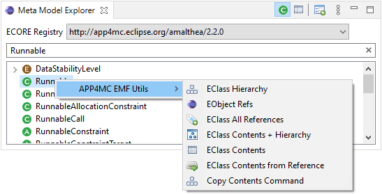
A double click on a list item shows an additional tree view with the hierarchy (sub classes and super classes) and all the attributes of the item. Multiple views can be opened in parallel.
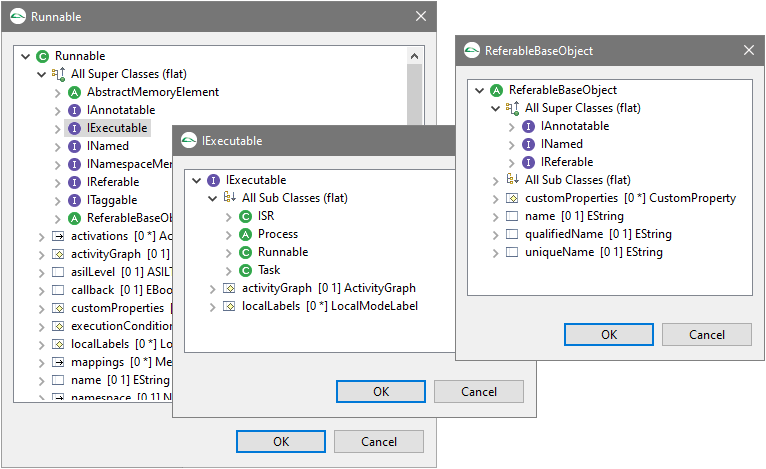
5.2.2 Graphical Viewer
The
Graphical Viewer shows SVG diagrams generated with PlantUML (https://plantuml.com). PlantUML is available as Eclipse plugin and will be installed automatically. The generation also requires GraphViz (http://www.graphviz.org/) that has to be installed manually.
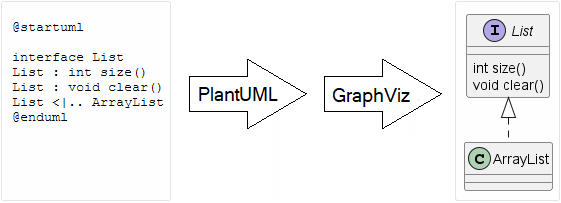
The generated diagrams are SVG files that are rendered by the browser component of SWT. The elements are also HTML links and can be used to navigate to diagrams of the same type but with a different selected element.
Some example diagrams:
Class Hierarchy
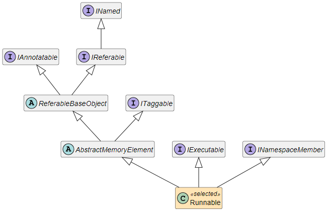
Class References
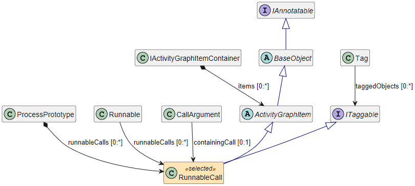
Class Hierarchy + Content
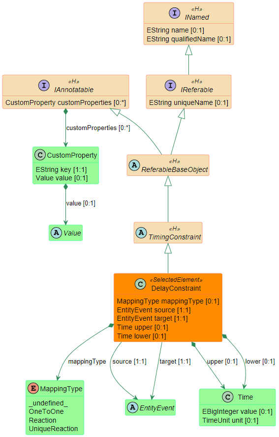
5.2.3 Installation via P2 update site
https://download.eclipse.org/app4mc/components/tools/emf-viewers/snapshot/p2repo
5.3 Additional Examples
5.3.1 IDE Extensions
Several APP4MC examples are already included in the APP4MC product.
They can be installed with the "New Examples Wizard" (New > Example...).
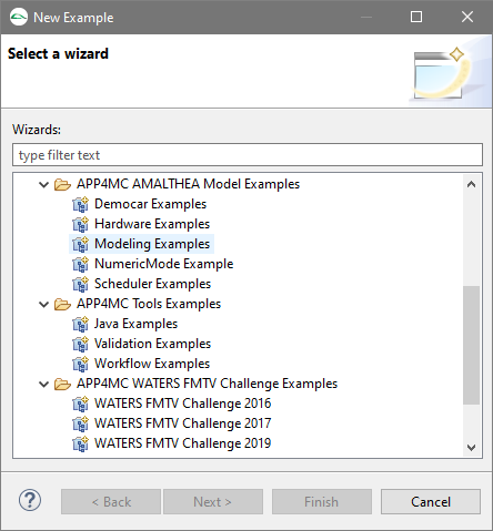
There are additional examples for
developers who want to extend the APP4MC platform.
The new example projects will be created as Plugin Projects in the current workspace. They can be modified and then tested in a separate runtime IDE.
-
IDE Actions example
- creates several new actions in the model editor:
- Add approval (for all elements that allow custom attributes)
- Convert to histogram (for Weibull-Distributions)
- Create C Type Definitions (in the software model)
-
IDE Validations example
- provides additional validations that can be checked on demand
-
IDE Visualizations example
- provides a demo visualization for elements that have a name attribute
Steps to install and test
1. Install additional examples via update site
https://download.eclipse.org/app4mc/updatesites/releases/3.0.0
https://download.eclipse.org/app4mc/updatesites/snapshot
2. Create example project(s)
3. Switch to Java perspective
4. Run a new Eclipse Application
Create a new Run Configuration to start another Eclipse instance ...
You can enter a name and start with the default settings...
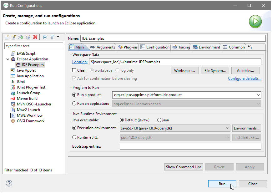
The new Eclipse runtime will contain all plugins of the current runtime and additional plugins based on the plugin projects in your workspace.
Therefore the created example projects extend the runtime IDE and the new features can immediately be tested.
5.4 Model Transformation
5.4.1 Transformation Framework
The transformation framework provides basic classes to perform transformations of EMF models. There are two possibilities: model-to-model (M2M) or model-to-test (M2T). The included examples show both cases.
Installation via P2 update site
https://download.eclipse.org/app4mc/components/addon/transformation/snapshot/p2repo
5.4.2 Generation of synthetic loads
The synthetic load generator (SLG) is a tool to generate synthetic C code that can be executed on a target platform. The generated code performs memory accesses and consumes runtime according to the specifications in the model. This allows the use of estimated or measured profiles for components that are not (yet) implemented. These generated parts of the system can run on the real hardware and enable early findings regarding the timing behavior of the overall system.
Installation via P2 update site
https://download.eclipse.org/app4mc/components/addon/transformation.slg/snapshot/p2repo/
5.4.3 Generation of SystemC code for simulation
The general timing simulation approach of an AMALTHEA model using APP4MC.sim is shown below. It consists of two steps, namely, transformation and simulation. The (model-to-text)
transformation step takes an AMALTHEA model as input and generates APP4MC.sim-specific code based on that model.
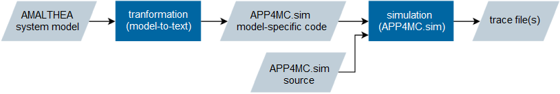
For a more detailed description of tool setup and usage please read section "SystemC Timing Simulation".
Installation via P2 update site
https://download.eclipse.org/app4mc/components/addon/transformation.sim.app4mc/snapshot/p2repo/
5.5 SystemC Timing Simulation
APP4MC.sim is a simulation framework for effective and early analysis of the runtime behavior of AMALTHEA models. It allows the consideration of software aspects and also the investigation of effects caused by concurrent accesses to shared hardware resources, especially memory in multi-core architectures. At its core, APP4MC.sim is based on the SystemC library with TLM extensions, which provides a solid foundation due to its widespread use and large user community.
External links:
General introduction
Step-by-step guide for the timing simulation of AMALTHEA models using APP4MC.sim
6 Release Notes
6.1 Eclipse APP4MC 3.3 (Jul 2024)
Model handling
- Model migration support (3.2.0 -> 3.3.0)
Product
- Target based on Eclipse IDE 2023-03
- Updated code compatibility and required execution environment to Java 17
- Several bug fixes
Minimum Java runtime is
Java 17.
6.2 Eclipse APP4MC 3.2 (Dec 2023)
Model handling
- Model migration support (3.1.0 -> 3.2.0)
Product
- Target based on Eclipse IDE 2022-03
- JavaFX 17 included (instead of JavaFX 11, still compatible with Java 11)
- Product definition with reduced scope (removed Xpand/Xtend, GEF, ...)
- Several bug fixes
Minimum Java runtime is
Java 11.
6.3 Eclipse APP4MC 3.1 (Jun 2023)
Model handling
- Model migration support (3.0.0 -> 3.1.0)
Product
- Updated frameworks: Visualization, Editor contribution
- New visualizations: Tag members, Event chains
- Updated visualization: Hardware structure
- IDE examples included in the standard distribution
- Several bug fixes
Minimum Java runtime is now
Java 11.
6.4 Eclipse APP4MC 3.0 (Nov 2022)
Model handling
- Model migration support (2.2.0 -> 3.0.0)
Model
- Removed deprecated model elements (ModeCondition* and ModeSwitch*)
- Simplified data type definitions (inline type definition is no longer supported)
- New lock type "Mutex"
- New lock attribute "ownership"
Product
- Extended model documentation and validation of semaphores
- Updated visualization framework:
- New utility classes for SVG (PlantUML, GraphViz)
- New persisted visualization parameters (per view)
- New visualization: EObject references
- Updated visualizations: Hardware, Runnable dependencies
- Several bug fixes
Recommended Java runtime is
Java 11.
Minimum is Java 8 (with limitations if JavaFX is not included).
6.5 Eclipse APP4MC 2.2 (Jul 2022)
Model handling
- Model migration support (2.1.0 -> 2.2.0)
- New utility functions (Stimuli event model)
Product
- Updated Runnable dependencies visualization
- Validations:
- New APP4MC.sim validations
- Duplicate ID check moved to EMF invariants (available as live validation)
- Extended help: Installable platform extensions
- Several bug fixes
Recommended Java runtime is
Java 11.
Minimum is Java 8 (with limitations if JavaFX is not included).
6.6 Eclipse APP4MC 2.1 (Apr 2022)
Model handling
- Model migration support (2.0.0 -> 2.1.0)
Model
- Extended ChannelFillCondition (attribute: relation)
- Extended relational operators (<=, >=)
- Added support for local mode labels
- Added ModeLabelEvent
Product
- New visualizations:
- Runnable dependencies
- Namespace members
- Validations: New APP4MC.sim validations
- Better handling of model compress / uncompress
- New preference settings (editor preferences)
- Several bug fixes
Recommended Java runtime is
Java 11.
Minimum is Java 8 (with limitations if JavaFX is not included).
For details see
Release 2.1.0 issues
6.7 Eclipse APP4MC 2.0 (Nov 2021)
Model handling
- Model migration support (1.2.0 -> 2.0.0)
Model
- Support for user extendible and clear scheduler definitions
- Extended condition handling
- New channel fill condition
Product
- New framework to extend model editor actions
- New model processing actions (e.g. cleanup)
- New creation of standard scheduler definitions
- Compress / uncompress of model files via context menu
- Several bug fixes
Developer resources
- Amalthea components (model, validation, migration) are available at
Maven Central
Recommended Java runtime is
Java 11.
Minimum is Java 8 (with limitations if JavaFX is not included).
For details see
Release 2.0.0 issues
6.8 Eclipse APP4MC 1.2 (Jul 2021)
Model handling
- Model migration support (1.1.0 -> 1.2.0)
Model extensions
- Activity graph
- added WhileLoop
- introduced non-interruptible groups
- Added nested elements (map) in custom properties
Product
- Improved Amalthea Model Editor
- Improved transformation BTF -> ATDB
- New model transformations (via "Install New Software...")
- New UI to start model transformations
- Several bug fixes
Developer resources
- Amalthea components (model, validation, migration) are now available at
Maven Central
Recommended Java runtime is
Java 11.
Minimum is Java 8 (with limitations if JavaFX is not included).
For details see
Release 1.2.0 issues
6.9 Eclipse APP4MC 1.1 (Apr 2021)
Model handling
- Model migration support (1.0.0 -> 1.1.0)
Product
- Improved handling of models in the Amalthea Model Editor
- model loading on demand
- faster loading of (large) models
- improved resolution of cross-file references
- Reduced dependencies of the Amalthea model
(allows easier use in non Eclipse environments)
- Removed "Amalthea no-load nature"
(no longer required because of model loading on demand)
- New visualization of scheduler mapping
- Validations: New APP4MC.sim validations
- Several bug fixes
Recommended Java runtime is
Java 11.
Minimum is Java 8 (with limitations if JavaFX is not included).
For details see
Release 1.1.0 issues
6.10 Eclipse APP4MC 1.0 (Nov 2020)
Model handling
- Model migration support (0.9.9 -> 1.0.0)
Model changes
- Removed MeasurementModel (deprecated since 0.9.9 and replaced by new ATDB)
- Removed ProcessEventType 'deadline'
Product
- New Amalthea Trace Database (ATDB)
- New transformations BTF -> ATDB, ATDB -> Amalthea
- Extended Metrics Viewer
- Several bug fixes
UI
- Added possibility to refresh a pinned visualization
For details see
Release 1.0.0 issues
6.11 Eclipse APP4MC 0.9.9 (Jul 2020)
Model handling
- Model migration support (0.9.8 -> 0.9.9)
Model changes
- Data types: Struct and StructEntry are tagable
- MeasurementModel is deprecated
Product
- Trace data and metrics: Extended definition of Amalthea Trace Database (Preview)
- Validations: New INCHRON validations, extended documentation
UI
- Model Explorer no longer expands model files
- Migration dialog supports recursive operation on folders
For details see
Release 0.9.9 issues
6.12 Eclipse APP4MC 0.9.8 (Apr 2020)
Model handling
- Model migration support (0.9.7 -> 0.9.8)
Product
- Eclipse target platform is updated to IDE 2019-12
- New (extendable) visualization framework
- Standard visualizations for runnables and deviations
- Additional example models
- EMF model viewers are available as update site
- ...
For details see
Release 0.9.8 issues
6.13 Eclipse APP4MC 0.9.7 (Jan 2020)
Model handling
- Model migration support (0.9.6 -> 0.9.7)
- Added virtual folders in component model tree view
Model changes
- Introduced namespaces and component structures
- New model element to describe hierarchical interfaces
- Model cleanup (simplified component ports)
Product
- Restructured migration component (also available as headless jar)
For details see
Release 0.9.7 issues
6.14 Eclipse APP4MC 0.9.6 (Oct 2019)
Model handling
- Model migration support (0.9.5 -> 0.9.6)
- New "no-load" nature (avoids model loading while moving/copying model files)
- Multi-line strings are supported in the editor (for selected string attributes)
Model changes
- Extended ModeConditions (allow the comparison of two mode labels)
- Refined EventChain definition (to explicitly describe fork-join, alternative, etc.)
- Counter added to RunnableCall
Build infrastructure
- Split git repository and independent build job for model migration component
- Changed to tycho-pomless maven builds
For details see
Release 0.9.6 issues
6.15 Eclipse APP4MC 0.9.5 (Jul 2019)
Model handling
- Model migration support (0.9.4 -> 0.9.5)
- New validation framework
Model changes
- Consolidated call graph: items of tasks and runnables are unified, call sequences are removed
- Simplified clock definitions (used in scenarios of variable rate stimuli)
- Limited frequency values to non negative (value >= 0)
For details see
Release 0.9.5 issues
6.16 Eclipse APP4MC 0.9.4 (Apr 2019)
Model handling
- Model migration support (0.9.3 -> 0.9.4)
- Optimized model search
- New validation framework (preview)
Model changes
- Extended modes to allow the handling of counters (integer values, comparison, increment, decrement)
- Uniform use of execution conditions (for stimuli, runnables, mode switches)
- Model cleanup (removed runnable deadlines, distinct naming)
For details see
Release 0.9.4 issues
6.17 Eclipse APP4MC 0.9.3 (Jan 2019)
Model handling
- Model migration support (0.9.2 -> 0.9.3)
- Optimized model search
Model changes
- Introduced "Ticks" as base concept for required computation effort
- Simplified "Execution Needs" (no specific entries for different processing units)
- Reworked distributions (discrete, continuous, time) without generics
For details see
Release 0.9.3 issues
6.18 Eclipse APP4MC 0.9.2 (Oct 2018)
Model handling
- Model migration support (0.9.1 -> 0.9.2)
- New model search dialog
- New model builders (with a Groovy-like builder pattern)
Model changes
- Small extensions in the hardware model
For details see
Release 0.9.2 issues
6.19 Eclipse APP4MC 0.9.1 (Jul 2018)
General
- New Eclipse Oxygen.3a based product (compatible with Java 8, Java 9 and Java 10)
- License change from EPL-1.0 to EPL-2.0
Model handling
- Model migration support (0.9.0 -> 0.9.1)
- New implementation of transient back references
- Unified approach for fast name search and mass delete
- Updated model utilities
Model changes
- New concept of DataDependency (to describe potential data dependencies)
- New possibility to specify RunnableParameters and CallArguments
6.20 Eclipse APP4MC 0.9.0 (Apr 2018)
Model handling
- Model migration support (0.8.3 -> 0.9.0)
- Updated model utilities
Model changes
-
New hardware model
- New concept of ExecutionNeed (replaces the former RunnableInstructions)
Note: This is the first implementation of the new hardware model. It will be extended in the next version and (minor) changes are expected.
6.21 Eclipse APP4MC 0.8.3 (Jan 2018)
General
- New Eclipse Neon.3 based product
Model handling
- Model migration support (0.8.2 -> 0.8.3)
- Updated model utilities
Model changes
- New mode conditions (logical AND)
- New timing requirement (end to start)
- Reworked Stimuli definitions
- New reference to port for client server and sender receiver communication
For details see
Release 0.8.3 issues
6.22 Eclipse APP4MC 0.8.2 (Oct 2017)
General
- Model changes (extensions)
- New graphical editors (based on Sirius)
Model handling
- Model migration support (0.8.1 -> 0.8.2)
- New model utilities
Model changes
- New runnable item to get the result of an asynchronous request
- New possibility to specify the label access implementation
- New measurement model
- New component event
For details see
Release 0.8.2 issues
6.23 Eclipse APP4MC 0.8.1 (Jul 2017)
General
- Model changes (extension and harmonization)
- Improved model handling
- New tooling: EMF Graphical Viewer
Model handling
- Model migration support (0.8.0 -> 0.8.1)
- New support for compressed model files (zip)
- More back references
Model changes
- Extended Schedulers (hierarchical, reservation based)
- Extend Semaphore definition (types)
- Consistent naming of Triggers, Activations and Stimuli
- New elements for data driven computation (conditions, triggers)
For details see
Release 0.8.1 issues
6.24 Eclipse APP4MC 0.8.0 (Apr 2017)
General
- Model changes (mainly to simplify handling)
- Improved tooling: model utilities
- New UI components: Multicore Wizard, Task-Visualizer (draft version)
Model handling
- Model migration support (0.7.2 -> 0.8.0)
Model changes
- Simplified model handling: Mapping Model, Modes, Time
- New classifiers to annotate Core and Memory
- Reworked Property Constraints
- Extended OS Overheads
For details see
Release 0.8.0 issues
6.25 Eclipse APP4MC 0.7.2 (Jan 2017)
General
- Smaller product definition (optional parts can be installed via update sites)
- Harmonized model API
Model handling
- Model migration support (0.7.1 -> 0.7.2)
- Improved back references
Model changes
- New core-specific runtimes (instructions) for runnables
- New model elements for streaming communication (Channels)*
- New Transmission Policy for communication (e.g. label accesses)
- New Event-based Stimulus
- New Data Consistency needs
- New Counters for InterProcessActivation and EventStimulus
- Harmonized model elements to describe probability
- Storage of common elements (e.g. tags) in one central location
Bug fixes / Improvements
- Model migration (ISR call graph, Section names, cross document references)
- Back references (Memory -> Mapping, Scheduler -> CoreAllocation)
Documentation
- New model elements: Physical memory sections, Channels
- New examples
* =
Experimental feature (first modeling attempt that may change in future versions).
For details see
Release 0.7.2 issues
6.26 Eclipse APP4MC 0.7.1 (Oct 2016)
Model handling
- Model migration support (0.7.0 -> 0.7.1)
- Improved update of opposite references
- Storage of default values is enabled by default
Model changes
- New distribution "Beta Distribution"
- New stimuli type "Synthetic" (to "replay" activations from a hardware trace)
- New DataStabilityGroup
- Introduced SamplingType as new attribute for Deviation
- Introduced physical memory sections (PhysicalSectionConstraint, PhysicalSectionMapping)
- Reworked AffinityConstraints (removed Scheduler constraints, added Data constraints)
- Reworked Event / Event-Chain Constraints
- Reworked RunnableSequencingConstraints
- New types for DataSizes and DataRates
For details see
Bugzilla entries for 0.7.1
6.27 Eclipse APP4MC 0.7.0 (Jul 2016)
Model handling
- Model migration support (itea1.1.0 -> itea1.1.1 -> 0.7.0)
- Simplified model creation wizard
- One consolidated model
- Additional opposite references (transient) to ease model navigation
- Scripting support for workflows (based on Eclipse EASE)
Model changes
- Removed 'attributes' and 'features' from hardware model
- Replaced generic
ProcessAllocation with specific
ISRAllocation and
TaskAllocation
- New
BigInteger values for
CustomAttributes
- Some renamed classes and attributes (details in the help)
Model structure
- Removed direct dependency to Franca (replaced by implicit reference by interface name)
Documentation
- Updated model documentation / class diagrams
- New developer guide regarding Model Migration Framework
- New developer guide regarding Workflows
7 Roadmap
Topics:
- Model changes (e.g. for heterogeneous hardware, Autosar adaptive)
- Model validation
- Model utilities
- Interactive help (visualization of model and meta model structure)
All releases are provided by
Eclipse APP4MC.
8 Frequently Asked Questions
8.1 Can APP4MC components be used in a pure Java environment?
Yes.
Amalthea components (model, validation, migration) are available at
Maven Central
9 Known Issues
9.1 Problem: UI freezes when a JavaFX visualization is invoked
The reason: Incompatibility of JavaFX and the glass.dll it tries to load when there are multiple Java versions available.
A simple solution: Add
-Djava.library.path= in the app4mc.ini after or before --add-modules=ALL-SYSTEM. This will avoid that Eclipse generates the value. As a result the java.library.path will be empty and JavaFX will load from the Java installation that was used to start APP4MC.
This issue mainly applies to older versions. It is already addressed in the product definition (since 2.1) and in the update site (since 3.0)
The longer explanation:
When Eclipse launches it automatically generates an entry for java.library.path that contains the path to the Java installation that is used to start Eclipse, and the PATH (on Windows it is the PATH system environment variable, not sure about the Linux equivalent). If additional Java installations are in the PATH, the java.library.path environment variable contains paths to multiple Java versions. It can then happen that JavaFX loads the glass.dll from the not matching Java installation (probably the one from Java 8 if APP4MC was started with Java 11), which then leads to NoSuchMethodErrors or similar that causes a crash.
There is already a
bug entry in Eclipse for that issue.
java.library.path is a Java environment variable that is used to add additional native libraries to the runtime. Typically only used in case native libraries should be added to an application that are loaded inside Java via System.loadLibrary(). As no additional external native libraries are required by APP4MC, setting java.library.path to an empty value should not have any effect on other functionalities. In Eclipse/OSGi development native libraries are typically included inside a plug-in project and do not reside external, as this would make the installation dependent on locally installed native libraries on the consumer side.