Eclipse LSAT™, Logistics Specification and Analysis Tool, is a tool for rapid design-space exploration of product logistics in flexible manufacturing systems. Eclipse LSAT™ has been developed by ESI (TNO) in collaboration with ASML and TU/e.
The tool enables lightweight modeling of system resources, system behavior, and timing characteristics. The tool provides various visualizations to explore the system behavior. Eclipse LSAT™ provides efficient performance analysis to compute the maximum system performance and to identify bottlenecks by exploiting the structure of the models.
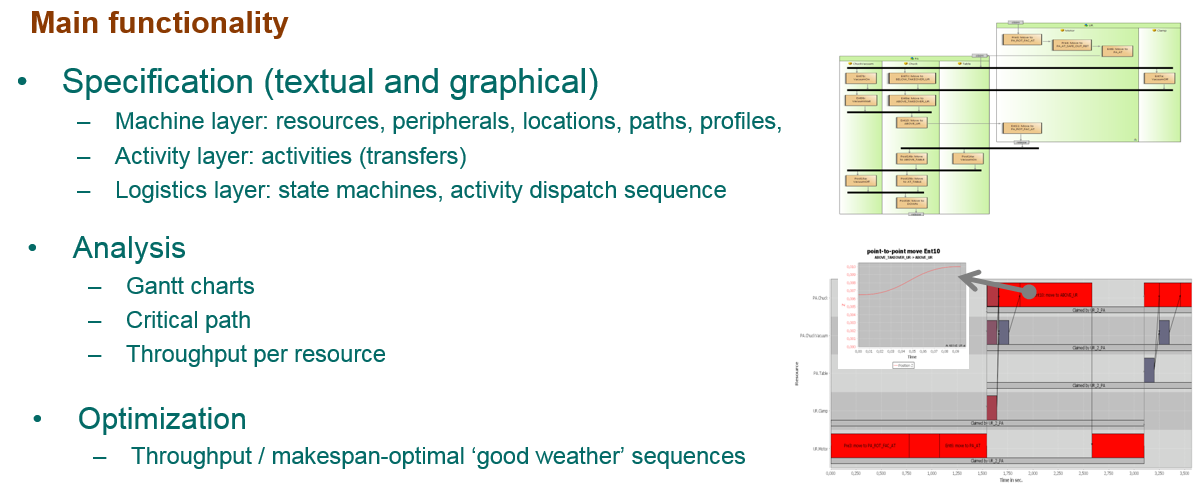
The figure below shows the main functionality of Eclipse LSAT™.
| The user guide can also be downloaded as a PDF. |
1. Eclipse LSAT™ IDE
1.1. Logistic perspective.
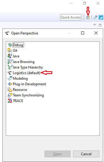
Once you have installed Eclipse LSAT™, you can choose the Logistics perspective following the instructions as below:
-
In Eclipse: select
-
Or, click to the icon of perspective (right-up of the window) and select Logistics as it is shown in the figure below:
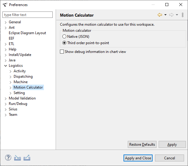
1.2. Motion Calculator
A motion calculator is used to calculate the time it takes for a move to complete. The default Third order point-to-point motion calculator is capable of calculating time for point-to-point moves with a 3rd order motion profile. It also supports passing moves, with the constraint that for all sub-moves the motion profile is the same.
Eclipse LSAT™ provides an extensible design for adding custom motion calculators. Creating a custom motion calculator requires knowledge about Eclipse plug-in development and Java. As such the instructions can be found in the design documentation of Eclipse LSAT™.
Eclipse LSAT™ also provides a simple JSON connector to add custom motion calculators written in other languages than Java. More details are provided in the design documentation of Eclipse LSAT™.
When a custom motion calculator is installed in the Eclipse LSAT™ environment, it can be selected via the menu.
2. Logistics Specification
2.1. Create New Project
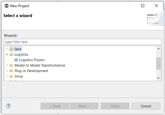
You can create a new specification by using the File > New menu on the Workbench menu bar. Start by creating a logistics project as follows:
-
From the menu bar, select File > New > Project…
-
In the New Project wizard, select Logistics > Logistics Project then click Next.
-
In the Project name field, type your name as the name of your new project, for example "Tutorial".
-
Leave the box checked to use the default location for your new project. Click Finish when you are done.
The wizard creates a machine specification in the project and configures the project for graphical editing. It will open the machine editor, allowing the user to add the resources and peripherals to the machine.
Within the project, the different types of specification can be created:
-
machine specification
-
settings specification
-
activity specification
-
activity dispatching specification
A new project always starts with machine specification, since it specifies the resources with their peripherals.
|
If it is the first time a file is created in the project, a pop up dialog about adding Xtext nature to the project will appear. Click Yes to continue. 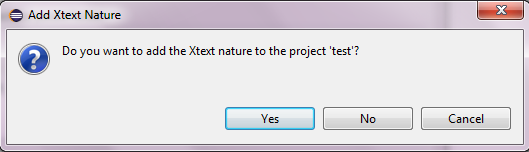
|
2.2. Create Machine Specification
Machine specification with file extension “machine” is used to specify the resources with their peripherals. This file is created automatically with the new project. It usually has the same name with the project, e.g. “tutorial.machine”.
A machine specification file can be opened to edit. Below are the basic concepts and small examples within a machine specification file.
| Ctrl+Space can be used to see the hints for the next step in textual editors. |
Machine Tutorial (1)

PeripheralType Clamp { (2)
  Actions {
    clamp
    unclamp
  }
}

PeripheralType Motor { (3)
  Actions {
    apply_brake
  }
  SetPoints {
    X [m]
    Y
  }
  Axes {
    X [mm] moves X
    Y [mm] moves Y
  }
  Conversion "X=X/1000;Y=Y/1000" (4)
}

Resource Robot1 { (5)
  C: Clamp
  M: Motor {
    AxisPositions { (6)
      X (Left, Right)
      Y (Above)
    }
    SymbolicPositions { (7)
      Above_Left (X.Left, Y.Above)
      Above_Right (X.Right, Y.Above)
      Below_Left (X.Left)
      Below_Right (X.Right)
    }
    Profiles (normal, slow) (8)
    Paths { (9)
      Above_Right --> Below_Right [Y] profile slow
      Below_Right --> Above_Right profiles normal, slow (10)
      Above_Left [X] <-> Above_Right profile slow
      FullMesh {
        profile normal
        Above_Left
        Above_Right
        Below_Left [Y]
      }
    }
  }
}
| 1 | Machine - the unique name for a machine |
| 2 | PeripheralType (unmovable) – it only declares actions |
| 3 | PeripheralType (movable) - it may declare actions, but it also declares set points and axes. The SetPoints relate to the physical coordinate system of the peripheral on which the motion profile settings are applied. The Axes relate to the symbolic coordinate system on which the physical locations are applied. An axis specifies which set points change when its value changes. The unit is specified between the square brackets [] and defaults to m(eters). |
| 4 | Conversion - If the unit of an axis differs from the unit of its set points a conversion script is required. The conversion needs to convert a physical location in the symbolic axes coordinate system to a physical location in the physical set points coordinate system. For each axis a variable is available containing its coordinate value and for each set point a variable should be set containing the set point value. NOTE: The script language is JavaScript |
| 5 | Resource – it defines its peripherals. For every movable peripheral in a resource its symbolic positions and paths need to be specified. |
| 6 | AxisPositions (optional) - if a peripheral has multiple axes and the symbolic positions can be categorized in axis positions, these axis positions may be declared in this section. In this case only a physical location per axis position is required in the settings file for this axis in stead of one location per symbolic position. |
| 7 | SymbolicPositions - declares the symbolic positions for this peripheral. Optionally a symbolic position may be expressed in its axes positions. If no axis position is specified (i.e. Below_Left and Below_Right) the symbolic position will automatically be added to the axis positions for the axis. |
| 8 | Profiles - declares the speed profiles to use for the paths. |
| 9 | Paths - declares which moves are allowed in the system. If a path is declared between two locations the move is allowed using the speed profile as specified by the path. For each end point of a path its settling axes can be specified as a comma separated list between square brackets []. Different types of paths are available: unidirectional path - indicated by an unidirectional arrow -->, only a move from left to right is allowed bidirectional path - indicated by a bidirectional arrow <->, both moves from left to right and right to left are allowed full mesh - indicated by keyword FullMesh, all moves from a location to another location in the full mesh are allowed. |
| 10 | Profiles - You can specify more than one speed profile per path by means of the profiles keyword. |
With the basic concepts as described above it is possible to make a full machine configuration.
2.2.1. Extended/Advanced Machine Specification
Machine configurations can be simplified, compressed or advanced using the concepts in below example:
import "tutorial.machine" (1)

Machine Tutorial

PeripheralType LinearMotor {
  SetPoints {
    X
  }
  Axes {
    X [mm] moves X
  }
  Conversion "X=X/1000"
}


PeripheralType FlipperType {
    SetPoints {
        C
    }
    Axes {
        C [mm] moves C
    }
    Conversion "C=C"
}

Resource Robot(give,take) { (2)
  C: Clamp
  M: LinearMotor {
    SymbolicPositions {
    	Home
    	Transfer
    	Flip

    }
    Profiles (normal, slow)
    Paths {
      Home <-> Transfer profile normal
      Transfer <-> Flip profiles slow, normal
    }
  }
}

Resource Flipper {
    C: Clamp
    F: FlipperType {
        Profiles (normal)
        Distances {     (3)
            HalfRound
        }
    }
}
| 1 | import - machine files can be split up into multiple files. |
| 2 | Resource items - multiple identical resources can be declared with identifiers (name or number) between parentheses (Robot.take, Robot.give in the example). |
| 3 | Distances - Instead of positions, distances can be specified. Distances only describe a move of a certain distance where the location is unknown or not relevant. Typically used for circular, belt or mill movements. Either (AxisPositions SymbolicPositions and Paths) or Distances must be specified. They are mutual exclusive. |
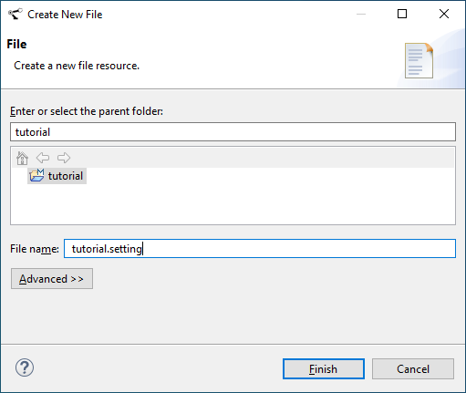
2.3. Create Settings Specification
Settings specification with file extension “setting” is used to specify physical settings for peripherals or peripheral actions. Within the project, create a “.setting” file by using the new file wizard.
| Multiple setting files are allowed in a project. They can be used to explore different system configurations |
| If another file is selected while running the new file wizard, this file will be automatically imported |
A setting file is opened. Below are the basic concepts in a settings file, illustrated with small examples.
| Ctrl+Space can be used to see the hints for the next step in textual editors. |
import "tutorial.machine" (1)

Robot1.M { (2)
  Timings { (3)
      apply_brake = 100e-3
  }
  Axis X {
    Profiles { (4)
      slow (V = 0.5, A = 0.5, J = 0.5, S = 0.1)
      normal (V = 1, A = 1, J = 1)
    }
    Positions { (5)
      Left (min = -100, max = -200, default = -150)
      Right = 300.0
    }
  }
  Axis Y {
    Profiles {
      slow (V = 0.5, A = 0.5, J = 0.5, S = 0.1)
      normal (V = 1.0, A = 1.0, J = 1.0, S = 0.1)
    }
    Positions {
      Above = 150.0
      Below_Left = -160.0
      Below_Right = -150.0
    }
  }
}

Robot1.C {
  Timings { (3)
    clamp = Normal(mean = 1.1, sd = 0.1)
    unclamp = 0.9
  }
}
| 1 | import - first step in a setting specification is to import a machine or other setting file. After that, it is allowed to specify properties for peripherals or actions. |
| 2 | Robot.M - for a movable peripheral, it is required to set the motion profiles to its profiles and physical relative locations to its symbolic positions. These properties are always set per axis. |
| 3 | Timings - if a peripheral contains actions, a timing must be specified. There are different types of timing available: Fixed value (no keyword) - One fixed value, use if the timing does not vary. Normal - The variation is specified using a normal distribution. Parameters: mean, sd (standard deviation) Triangular - A triangular distribution as described here. Parameters: min, max, mode. Pert - A Pert distribution as described here. Parameters: min, max, mode, gamma. NOTE: In addition to the distribution specific parameters, it is possible to specify a default value for a distribution. If present this value is used for scheduling. The distributions are used for stochastic impact analysis. If no default is specified the mode of the distribution will be used. |
| 4 | Profiles - motion profiles need to be assigned to each profile individually. For the built-in motion calculator they can be either Third-order profile (VAJ) or Second-order profile (VA). Optionally a settling time (S) can be specified per profile. |
| 5 | Positions - physical relative locations can be specified as a set of maximum, minimal and default values or one fixed value. |
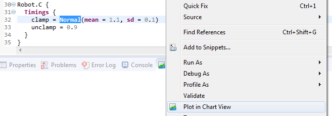
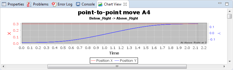
2.3.1. Plotting a timing distribution
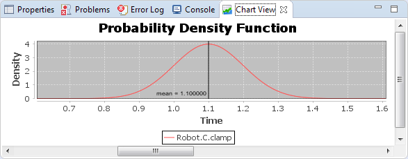
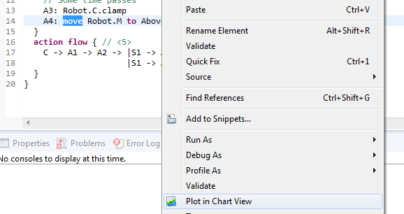
To gain insight in the probability density for timings in a distribution, the probability density factor (PDF) can be plotted in the Chart View. To do this, please select the distribution keyword of the requested distribution and select the 'Plot in Chart View' item from the context menu, as illustrated in the next figures
| The chart view also shows the mean marker, this is the value used for scheduling. |
2.3.2. Extended/Advanced Settings Specification
Setting files can be advanced using Expressions and/or combined Resource items:
import "tutorial_ext.machine"
import "tutorial.setting"

// area settings.
val width = 300   (1)
val height = 300
val right = width/2  (2)
val left = width/-2
val homeLeft = left - 10
val homeRight = right + 10
val center = (right - left)/2
// timings
val breakTiming = 100e-3

//profiles (artificial)
val vRSlow = 0.5
val aRSlow = 0.5
val jRSlow = 0.5
val sRSlow = 0.1
val vRNormal = vRSlow*2
val aRNormal = vRSlow*2
val jRNormal = vRSlow*2
val sRNormal = 0.1
val clampLow = 1
val clampSD = 0.1

Robot.give.M { (3)
  Axis X {
    Profiles {
      slow (V = vRSlow, A = aRSlow, J = jRSlow, S = sRSlow) (4)
      normal (V = vRNormal, A = aRNormal, J = jRNormal)
    }
    Positions {
      Transfer = left
      Home = homeLeft
      Flip = center
    }
  }
}

Robot.take.M { (3)
  Axis X {
    Profiles {
      slow (V = vRSlow, A = aRSlow, J = jRSlow, S = sRSlow)
      normal (V = vRNormal, A = aRNormal, J = jRNormal)
    }
    Positions {
      Transfer = right
      Home = homeRight
      Flip = center
    }
  }
}

Robot.C { (5)
  Timings {
    clamp = Normal(mean = clampLow+clampSD, sd = clampSD)  (6)
    unclamp = 0.9
  }
}

Flipper.F {
    Axis C {
        Profiles {
             normal (V = 1, A = 1, J = 2)
        }
        Distances {  (7)
            HalfRound = 0.5
        }
    }
}

Flipper.C {
  Timings {
    clamp = 0.5
    unclamp = 0.9
  }
}
| 1 | Expressions - instead of magic numbers Expressions can be used. Re-usable Expressions can be declared immediately after the import statement(s). |
| 2 | Calculations - simple calculations using * / - + and parentheses are supported. |
| 3 | Different settings for Resource items - Place the identifier as specified in the machine file between the Resource and the Peripheral to make specific settings for a Resource item (In this example: Robot.give.M). |
| 4 | Usage - Expressions can be used to calculate the actual properties. |
| 5 | Resource items - multiple resources with identical Peripheral settings can be specified using the Resource name. |
| 6 | Expressions in assignments - Expressions calculations can directly be used in assignments. |
| 7 | Distances - when using distances the Distance must be specified as described. |
| Hovering over an Expression or an assignment yields the calculated result in a pop-up window. |
| For a Peripheral within a Resource, settings must be specified for either the Resource or all Resource items. An error will be raised if a combination is made. |
Explore different settings.
Similar to machine files, setting files can also be split up into multiple files. import of machine and other setting files is supported. In Create Activity Dispatching Specification is described how to choose different setting files.
2.4. Create Activity Specification
Activity specification with file extension “activity” is used to specify activities of a machine. Within the project, create an “.activity” file by using the new file wizard.
| If another file is selected while running the new file wizard, this file will be automatically imported |
An activity specification file is opened. Below are the basic concepts and small examples within a activity specification file.
| Ctrl+Space can be used to see the hints for the next step in textual editors. |
import "tutorial.machine" (1)

activity MoveRobot { (2)
  prerequisites { (3)
    Robot1.M at Above_Right
  }
  actions { (4)
    C: claim Robot1
    R: release Robot1
    A1: move Robot1.M to Below_Right with speed profile slow
    A2: Robot1.C.unclamp
    // Schedule A3 to end together with A4 (As Late As Possible)
    A3: Robot1.C.clamp ALAP (5)
    A4: move Robot1.M to Above_Right with speed profile normal
  }
  action flow { (6)
    C -> A1 -> A2 -> |S1 -> A3 -> |S2 -> R
                     |S1 -> A4 -> |S2 (7)
  }
}
| 1 | import - first step in an activity specification is to import a machine specification file. |
| 2 | activity - specify activities by defining individual actions and dependencies among these actions. |
| 3 | prerequisites - specify the initial location for all movable peripherals for this activity. |
| 4 | actions - there are four types of actions:
|
| 5 | ALAP / ASAP - Each action has scheduling type.
There are two types available: As Soon As Possible (ASAP) and As Late As Possible (ALAP).
If no value is specified at the end of the action, then the scheduling type is ASAP by default.
To change it to ALAP you can add the ALAP keyword at the end of the action.
For more information, see section Constraints for ALAP and ASAP scheduling actions. Resource claiming – ASAP by default, but will be ALAP if required by peripheral actions, cannot be changed. Resource releasing – ASAP by default, cannot be changed. Peripheral action – ASAP by default, can be changed to ALAP. Move - ASAP by default, can be changed to ALAP. |
| 6 | action flow - uses arrows to specify action flow. A1 → A2 represents A2 starts when A1 finishes. |
| 7 | syncbar - used to specify synchronization, for instance A2 → |S1 → A3 and |S1 → A4 represents A3 and A4 start simultaneously after A2 finishes. |
2.4.1. Extended/Advanced Activity Specification
Distance moves and resource items can be used in activities, as specified below:
import "tutorial_ext.machine"

activity MoveAndFlip {
  prerequisites {
    Robot.give.M at Transfer
    Robot.take.M at Transfer
  }
  actions {
    RGClaim: claim Robot.give (1)
    RGRelease: release Robot.give
    FClaim: claim Flipper
    FRelease: release Flipper
    RTClaim: claim Robot.take
    RTRelease: release Robot.take
    RGMoveFlip: move Robot.give.M to Flip with speed profile normal
    RGMoveTransfer: move Robot.give.M to Transfer with speed profile slow
    RTMoveFlip: move Robot.take.M to Flip with speed profile normal
    RTMoveTransfer: move Robot.take.M to Transfer with speed profile slow
    RTClamp: Robot.take.C.clamp
    RTUnclamp: Robot.take.C.clamp
    RGClamp: Robot.give.C.clamp
    RGUnclamp: Robot.give.C.unclamp
    FFlip: move Flipper.F for HalfRound with speed profile normal (2)
    FClamp: Flipper.C.clamp
    FUnclamp: Flipper.C.unclamp
  }
  action flow {
    RGClaim -> RGClamp -> RGMoveFlip -> FClaim->FClamp -> RGUnclamp -> |S1 ->FFlip -> |S2
    RTClaim -> RTMoveFlip -> |S2
    |S1 -> RGMoveTransfer -> RGRelease
    |S2 -> RTClamp -> FUnclamp -> FRelease-> RTMoveTransfer -> RTUnclamp -> RTRelease
  }
}

activity RobotStart {  (3)
  prerequisites {
    Robot.M at Home
  }
  actions {
    Claim: claim Robot
    Release: release Robot
    MoveTransfer: move Robot.M to Transfer with speed profile normal
  }
  action flow {
    Claim -> MoveTransfer ->  Release
  }
}

activity RobotStop { (3)
  prerequisites {
    Robot.M at Transfer
  }
  actions {
    Claim: claim Robot
    Release: release Robot
    MoveHome: move Robot.M to Home with speed profile normal
  }
  action flow {
    Claim -> MoveHome ->  Release
  }
}
| 1 | Resource item - In an activity a resource item can be specified by the resource name followed by the identifier (Robot.give in the example). |
| 2 | Distances a distance move is specified with the for keyword instead of to. In case of a passing move use the keyword continuing instead of passing. For distances an initial position cannot be specified. |
| 3 | Resource - An activity can also refer to a resource, without specifying the specific resource item. The advantage of this is that the activity specification can be reused and instantiated for the specific resource items. The specific resource item is assigned in the activity instance in the activity dispatching specification. See Extended/Advanced Activity Dispatching Specification for an example. |
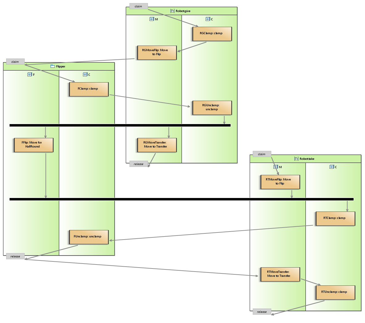
| The shown activity is an activity that brings a product from left to right using 2 robots. The product is flipped in the center. Graphically it looks as follows: |
2.4.2. Constraints for ALAP and ASAP scheduling actions
There are a number of validation rules implemented in Eclipse LSAT™ for the different scheduling algorithms. In general you have to keep two things in mind:
-
The scheduler algorithm prefers ASAP scheduling over ALAP scheduling.
-
A concatenated move with events on-the-fly may be delayed as a whole, but not in between its events.
Scenario 1
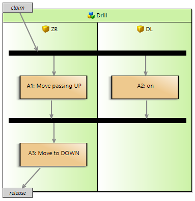
Consider action A1 in the ALAP scenario 1 with scheduling type ALAP and a sole successor (A2), which is not a syncbar. In this case the ALAP keyword does not have any effect due to the ASAP (default) scheduling of action A2.
Eclipse will show you the following warning:
| The ALAP keyword does not have any effect for action A1. |
Scenario 2
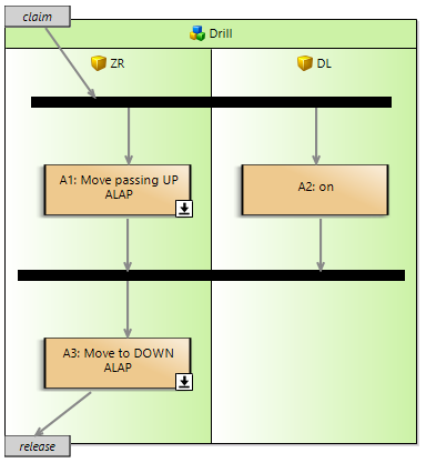
Consider move A1 in ALAP scenario 2 which is passing. As its successor is a syncbar, and this syncbar has more than one predecessor, then move A1 must be ALAP. As moves A1 and A3 should be concatenated, there cannot be any delay between them. As action A2 might cause such a delay, move A1 needs to be scheduled ALAP to guarantee concatenation.
Eclipse will show you the following error:
| Move A1 must be set to ALAP to guarantee concatenation with successor move A3. |
Scenario 3
Consider move A3 in ALAP scenario 3 which is a continued move of A1. Move A1 continues into move A3 by means of the passing keyword and therefore move A3 cannot be delayed. As the predecessor of move A3 is a syncbar, move A3 must be ASAP to guarantee concatenation.
Eclipse will show you the following error:
| Move A3 must be set to ASAP to guarantee concatenation with predecessor move A1. |
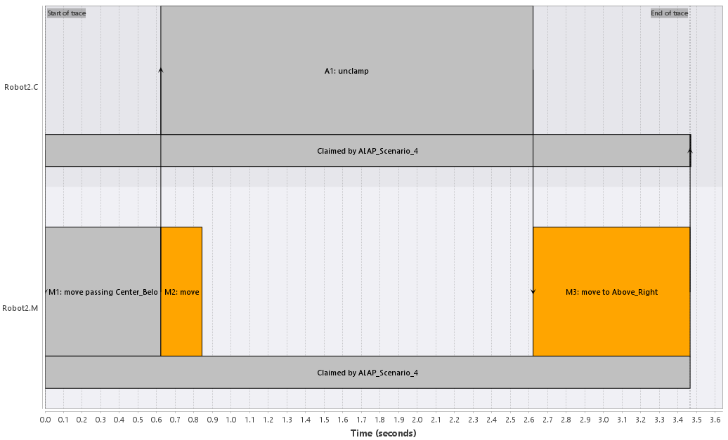
Scenario 4
Consider move M3 in ALAP scenario 4 which is a continued move of M1 and M2.
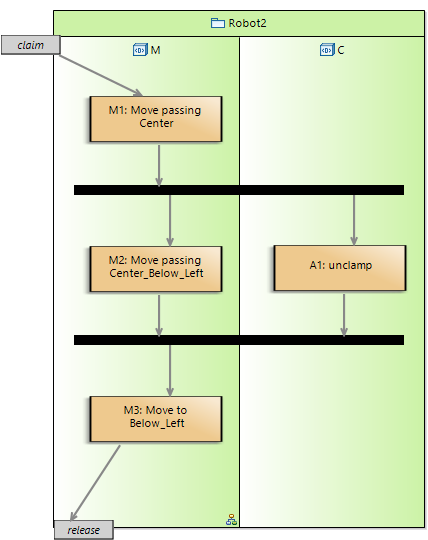
Move M2 finally continues into move M3 by means of the passing keyword and therefore move M3 cannot be delayed. Because action A1 is parallel to M2 this cannot be guaranteed hence to following warning will be shown:
| Parallel action 'A1' might interrupt concatenated move 'M3'. |
If after a Timing analysis it appears that M3 is indeed delayed the following error will be shown:
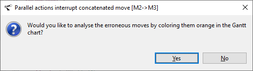
In the ALAP scenario 4 Gantt chart the erroneous move is colored orange.
2.5. Create Activity Dispatching Specification
Activity dispatching specification with file extension “dispatching” is used to specify a sequence of activities to schedule. For more information about scheduling, see section Schedule Activities. Within the project, create a “.dispatching” file by using the new file wizard.
An activity dispatching file is opened. Below are the basic concepts and small examples within a activity dispatching file.
| Ctrl+Space can be used to see the hints for the next step in textual editors. |
import "tutorial.activity" (1)

throughput {
	iterations: 1 (2)
	iterations.Robot1: 2
}

activities { (3)
  MoveRobot ("First product")
}

activities {
  offset: 6.00 (4)
  MoveRobot ("Second product")
}
| 1 | import - first step in an activity dispatching is to import an activity specification file. |
| 2 | iterations - specifies the default number of iterations - for all resources - or the number of iterations for a specific resource (see next line). When omitting the throughput section the default number of iterations will be set to 1. For more information about iterations see section Specifying the number of iterations. |
| 3 | activities - within an activity sequence one or more activities can be included. These activities will be scheduled as parallel as possible adhering to the claim/release strategy. If activities cannot be scheduled in parallel the order of this section is applied. Optionally a description can be added to the activity |
| 4 | offset - optionally an offset can be defined for an activity sequence. The scheduler will ensure that these activities will not be started before the offset time. |
2.5.1. Extended/Advanced Activity Dispatching Specification
import "tutorial_ext.activity" (1)

activities rampUp { (2)
  RobotStart[give] (3)
  RobotStart[take]
}

activities steadyFlow(anAttribute:1) (4)
  repeat coin: [2,4] { (5)
  yield: 1  (6)
  MoveAndFlip(step:1,scenario:"normal") (7)
  MoveAndFlip(step:2,scenario:"normal")
}

/** steady flow expands to:
activities steadyFlowExpanded(anAttribute: 1) {  (8)
    yield: 2
    MoveAndFlip(step: 1, scenario: "normal", phase: steadyFlow, coin: 2)
    MoveAndFlip(step: 2, scenario: "normal", phase: steadyFlow, coin: 2)
    MoveAndFlip(step: 1, scenario: "normal", phase: steadyFlow, coin: 4)
    MoveAndFlip(step: 2, scenario: "normal", phase: steadyFlow, coin: 4)
}
*/
activities tearDown { (2)
  RobotStop[give]
  RobotStop[take]
}
| 1 | import - import one or more activity files. |
| 2 | activity phase - a phase name may be specified to indicate a specific phase like start-up, steady-flow, or tear-down. |
| 3 | resource item - for activities that have their specific resource item not yet specified the resource item must be specified (For example: The RobotStart activity will be performed for the give and take robot). |
| 4 | user attributes - user info can be added for an activity. This information will be passed to the trace file see Schedule Activities. |
| 5 | repeat - the number of time these activities need to be scheduled. This will be visible in the Schedule Activities. By default 1. |
| 6 | yield - the number of products one repeat of activities yields. |
| 7 | user attributes - attributes that will be assigned to the activity instance. |
| 8 | the steadyFlow activity is functionally equal to steadyFlowExpanded. |
| user attributes, activity phase, repeat step (and also activity trace points) are all stored in a generated Gantt Chart. See also Schedule Activities |
2.5.2. Specifying the number of iterations
The number of iterations is used to calculate the throughput per resource, as explained in section Calculating the Throughput per Resource. In the activity dispatching specification example above the Robot resource performs activity MoveRobot twice, once for the "first product" and once for the "second product". In this case the number of iterations can be used for the calculation on how many products per hour can be processed by the Robot resource.
| The number of iterations does not influence the Schedule Activities or Conformance Check. |
| throughput is now deprecated and can be replaced with repeat and yield as described in Extended/Advanced Activity Dispatching Specification. |
2.6. Create Supervisory Controller Specification
A specification with an individual activity sequence can be described in a "dispatching" specification, see Create Activity Dispatching Specification. A CIF specification is used to concisely describe a supervisory controller that defines all allowed activity sequences that establish a correct product flow, while taking into account product routing flexibility.
In a CIF specification, a network of automata is used as formalism. The outgoing edges in an automaton refer to the allowed activities in the given automaton location. Multiple edges represent a scheduling choice where multiple activities are allowed. Automata are synchronized on the activity names with multi-party synchronization. This means that an activity can only be executed in the current system state, if it is enabled in the current state of each of the synchronizing automata.
A small example of a supervisory controller is shown below.
controllable MoveRobot; (1)

supervisor Tutorial: (2)

  location l0:
    initial; (3)
    edge MoveRobot goto l1; (4)

  location l1:
    edge MoveRobot goto l0;

end
| 1 | controllable - specifies all activities that are used in the specification, separated by commas. |
| 2 | supervisor - the name of the supervisory controller |
| 3 | initial - indicates the starting location of the supervisory controller |
| 4 | edge - indicates that activity MoveRobot can be executed from location l0, leading to location l1. |
A supervisory controller can also be generated from a set of requirement and plant automata. The plant automata specify all allowed activity orderings, and the requirements put constraints on the ordering of activities to establish the correct product flow. Using supervisory controller synthesis, a supervisory controller is generated that enforces the requirements and ensures that the system does not deadlock. The documentation and tutorials for CIF, including how to use supervisory controller synthesis, can be found at https://www.eclipse.org/escet.
3. Graphical Viewers
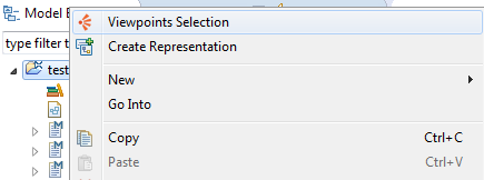
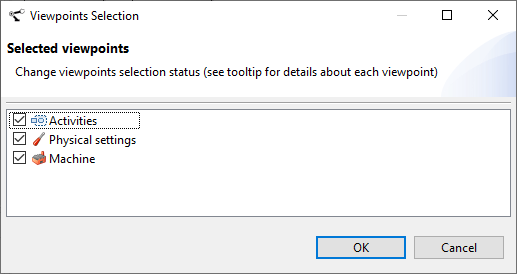
3.1. Add Viewpoints Selection
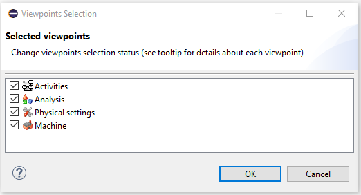
Right click on the project folder, select Viewpoints Selection.
The following viewpoints are available:
| Machine |
shows the resources with their peripherals and illustrates symbolic position graphs for movement-based peripherals. |
| Activities |
shows activity diagrams based on activity specifications. |
| Physical settings |
shows settings for motion profiles and physical locations. |
Check the relevant viewpoints and click OK.
3.2. Generate Graphs
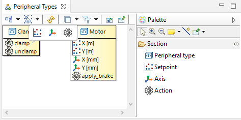
3.2.1. Peripheral types in machine
Target element: a machine
Right click on a target element, select New Representation and choose the corresponding Peripheral Types for the target element.
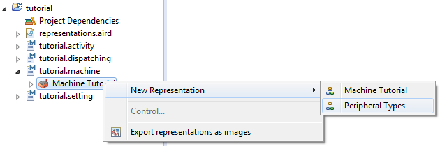
The peripheral types graph for the target element includes all action and movement based peripheral types for the target element.
| This viewer can also be used to edit the peripheral types by using the palette. |
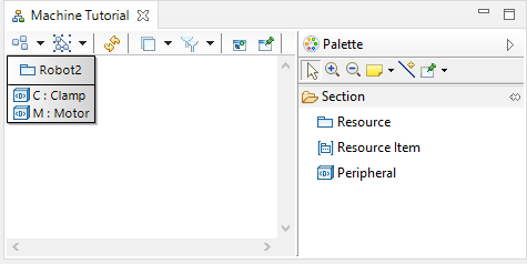
3.2.2. Resources and peripherals in machine
Target element: a machine
Right click on a target element, select New Representation and choose the corresponding Machine for the target element.
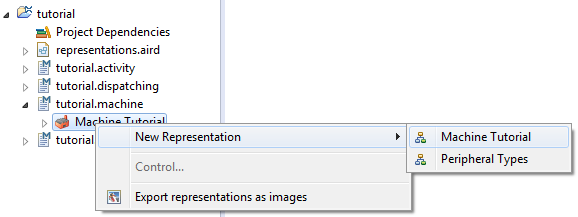
The graph for the target element includes all resources with their action-based and movement-based peripherals for the target element.
| This viewer can also be used to edit the resources and their peripherals by using the palette. |
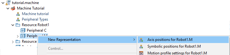
3.2.3. Axis position graph for peripheral
Target element: a movable peripheral defined in a resource
Right click on a target element, select New Representation and choose the corresponding Axis positions for the target element.
The axis position graph for the target element includes specific information about axes and corresponding positions.
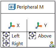
The axes in a axis position graph are shown as compartments, and the positions associated to an axis are shown under the axis. For example, in the figure above, the position Above is associated to the axis Y.
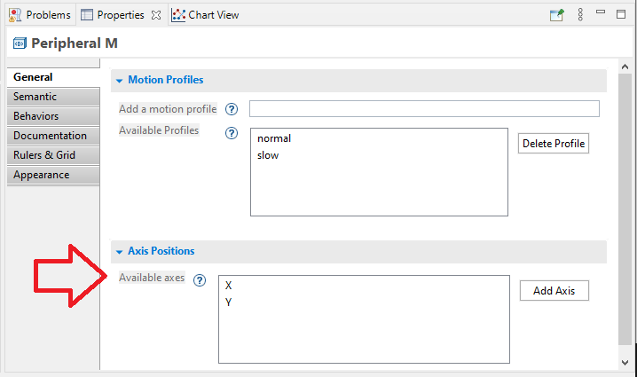
Adding/removing axes
To add a new axis to a peripheral, select the empty canvas and select the desired axis from the Available axes list in the properties view. Press Add Axis on the right side.
To remove an axis from a peripheral, select it and press Delete.
| Deleting an axis will also delete all corresponding positions. |
Adding/deleting positions
The positions can be associated to an axis by selecting the Position tool from the Axis Positions Editor Tools palette on the right side, and selecting the axis compartment.
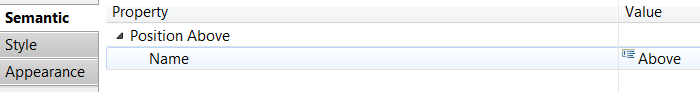
By default, name of the newly created position is new. The name of a position can be changed by selecting it, typing the name directly and pressing Enter. Alternatively, the name can be changed using the properties editor, as shown in the figure below.
To delete a position, select it and press Delete.
| If a position is specified in both axis position graph and Settings Create Settings Specification, deleting that position from the axis position graph will also delete it from the Settings specifications. |
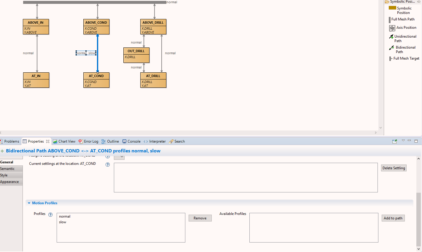
3.2.4. Symbolic position graph for peripheral
Target element: a movable peripheral defined in a resource
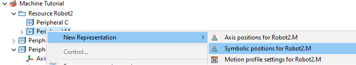
Right click on a target element, select New Representation and choose the corresponding Symbolic positions for the target element.
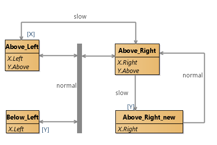
The symbolic position graph for the target element includes specific information about profiles and settling on the paths.
| Layout of existing symbolic position graphs will be reset to default layout. As manual layout of these diagrams may require extra time and labor, it may not be wise to upgrade to the latest release of Eclipse LSAT™ for existing symbolic position specifications. |
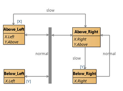
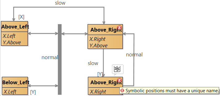
The symbolic positions are shown as compartments. The axis positions corresponding to a symbolic position are shown inside the respective compartment.
The full mesh paths are shown as gray vertical rectangles. The single-headed arrows between symbolic positions represent unidirectional paths, whereas double-headed arrows represent bidirectional paths. If a symbolic position is a part of a full mesh path, then there is also an arrow between the symbolic position and the full mesh path.
The labels in the center of paths represent motion profiles. Whereas, the labels at the end of paths represent settling.
Adding/deleting motion profiles
To add a new motion profile to a peripheral, click on the empty canvas. As a result, properties editor will appear at the bottom. Enter the name of the motion profile without a white space in the field Add a motion profile, as shown in the following figure, and hit Enter.
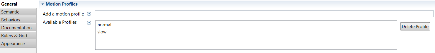
The available profiles are visible in the Available Profiles field. To delete a profile, select it and press Delete Profile on the right side.
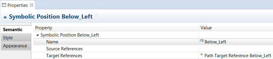
Adding/deleting symbolic positions
To create a new symbolic position, select the respective tool from the Symbolic Positions Editor Tools palette on the right side, and then click on the canvas. The name of the symbolic position can be typed directly while selecting the newly created symbolic position. Alternatively, the name can also be typed in the properties editor at the bottom, as shown in the following figure.
To delete a symbolic position, select it and press Delete.
Adding/deleting axis positions
The axis positions can be added to a symbolic position compartment by selecting the respective tool and selecting the symbolic position compartment. The name of the axis position can be typed directly in the format Axis.Position (same as textual representation). Alternatively, the name can also be typed in the properties editor at the bottom, as shown in the following figure. Here, Key represents an axis and Value represents a position. To delete a axis position, select it and press Delete.
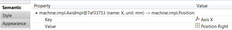
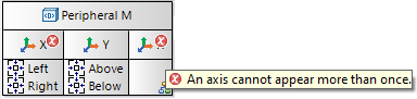
| The typed axis position name cannot be entered if either of the typed axis or position does not exist. |
Adding/deleting paths
Uni/bidirectional paths between two symbolic positions can be added by selecting the respective tool and clicking the symbolic positions. To add a symbolic position to a full mesh path, select the Full Mesh Target tool, and then click the full mesh path and the symbolic position. To delete a path, select it and press Delete.
A settling to a unidirectional path can be added in the properties editor by selecting the path, as shown in the figure below.
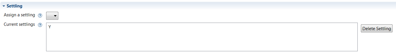
In the Assign a settling field, a settling can be selected for a path. The settlings currently assigned to a path are visible in the Current settlings field. To remove a settling from a path, first select the path and then select the settling in the Current settlings field and press Delete Settling on the right side.
In bidirectional paths, we can add two settlings, i.e., one settling for each connected symbolic position. A settling to a bidirectional path can be added in the properties editor by selecting the path, and then assigning a settling at each connected symbolic position, as shown in the figure below.
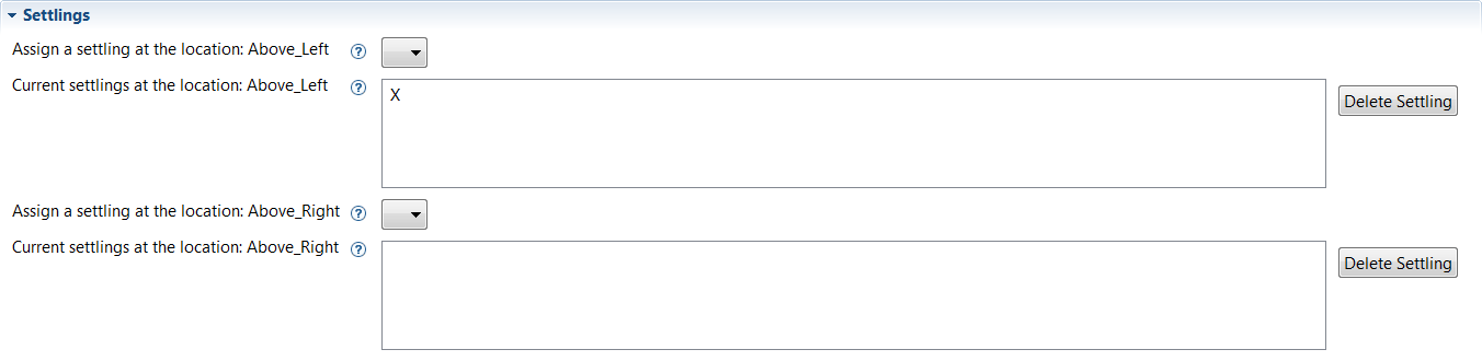
The settlings currently assigned to a path at a symbolic position are visible in the Current settlings field. To remove a settling from a path, first select the path and then select the settling in the Current settlings field and press Delete Settling on the right side.
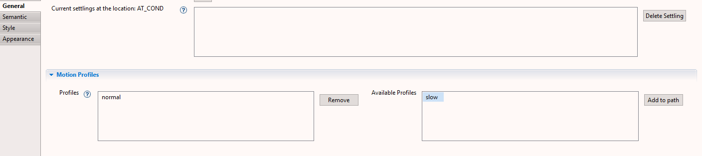
Assigning existing motion profiles to a path
To add a motion profile to a path, choose one of the options below:
- Option I
-
-
Select the path by left clicking on it.
-
Select the General tab.
-
Scroll down to the Motion Profiles section.
-
Select your the profile you want to add from the Available profiles list.
-
Press Add to path.
-
- Option II
-
-
Select the motion profile from the diagram by left clicking on it.
-
Press F2 to enable direct editing.
-
Add a comma after the existing profile and write the name of the profile you want to add, e.g normal, slow .Please note slow should have been initialized earlier.
-
Save your diagram. The changes are then saved to the model.
-
Hiding axis positions/paths
In order to visualize a diagram clearly, it is possible to hide axis positions or paths or both from a diagram. To hide axis positions, click on the canvas, and then click on the Filter icon on the top tool bar, and click Axis Positions, as shown in the figure below.
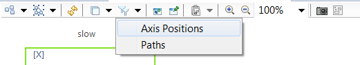
Paths from a diagram can also hidden in the same way.
Layout
A symbolic position graph can be layout by right clicking on the canvas and selecting Show Layout View.
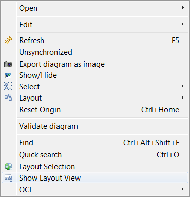
As a result, a new tab named Layout will appear at the bottom. Click on the empty canvas, and then in the Layout tab, a new Property Layout Algorithm with a Value Activity Diagram will appear.
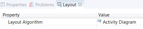
Select Activity Diagram, and double click it or use the button on the right side.
A pop-up will appear showing all pre-defined layout algorithms. In our experience, the ELK Layered algorithm is most suitable for symbolic position graphs. However, please feel free to explore other algorithms also.
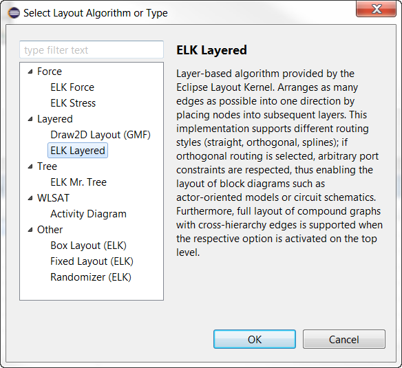
Select an algorithm and press OK. Afterwards, apply the automatic layout by right clicking on the canvas and selecting Layout Selection from the context menu, or use the button from the toolbar  .
.
Validation
Each symbolic position must have a unique name. To validate this property, right click on the canvas and click Validate diagram. If any symbolic positions do not have unique names, a red error sign will appear on those symbolic positions, as shown in the following figure.
To quickly fix this error, a quick fix is available. Go to the Problems tab on bottom and right click on the error message and select Quick Fix, as shown in the figure below.
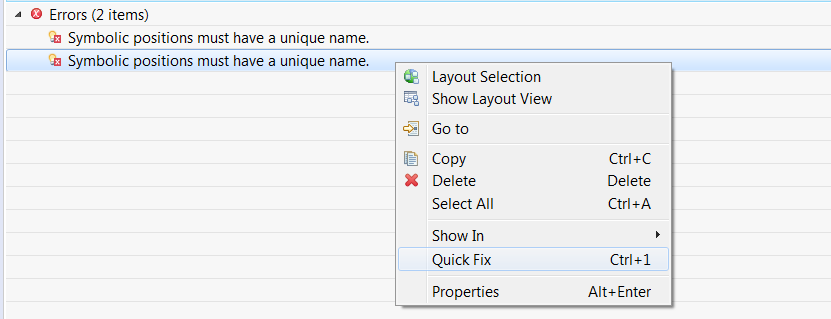
Then select the Change name and press Finish.
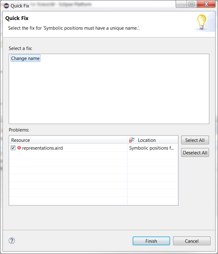
As a result _new will be added at the end of the name of the symbolic position.
3.2.5. Motion profile settings table for peripheral
Target element: a movable peripheral defined in a resource.
Right click on a target element, select New Representation and choose the corresponding motion profile for the target element.
| If the representation is not listed in the context menu, most likely the physical settings viewpoint needs to be activated for the project, see Add Viewpoints Selection. |
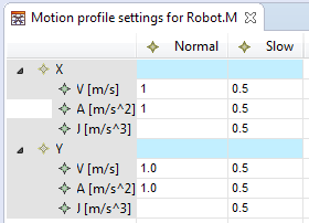
Motion profile settings data is from the first setting file in the project directory.
Column specifies profile names and row represents one axis. Each row contains sub rows to specify VAJs for an axis.
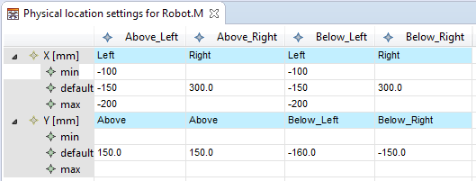
3.2.6. Physical location settings table for peripheral
Target element: a movable peripheral defined in a resource.
Right click on a target element, select New Representation and choose the corresponding physical location settings for the target element.
| If the representation is not listed in the context menu, most likely the physical settings viewpoint needs to be activated for the project, see Add Viewpoints Selection. |
The same to motion profile settings table, the physical location settings data is also from the first setting file in the project directory.
In the table, each column represents one symbolic position for the target element. Each row represents its axes and the physical location values (min, default, and max) are shown on the sub rows.
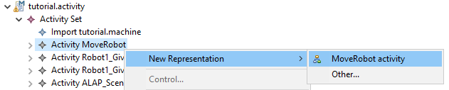
3.2.7. Activity diagram
Target element: an activity defined in an activity specification
Right click on a target element, select New Representation and choose the corresponding activity for the target element.
| If the representation is not listed in the context menu, most likely the activities viewpoint needs to be activated for the project, see Add Viewpoints Selection. |
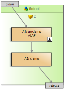
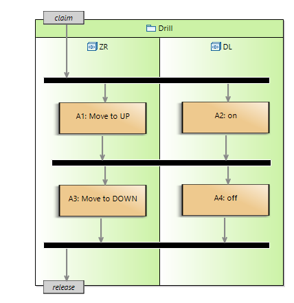
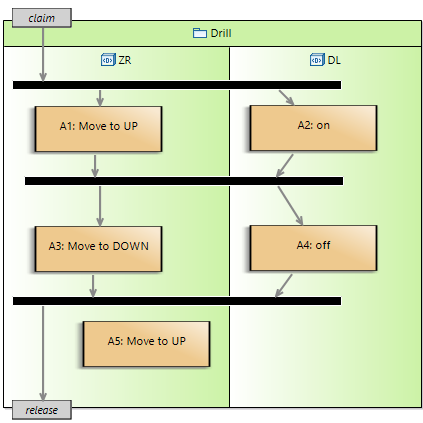
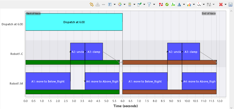
It shows an activity diagram with an action flow. Green swim-lanes represent
resources and their peripherals, gray blocks represent
either claiming a resource or releasing a resource and brown blocks
represent actions for peripherals.
If an action is specified to be scheduled As Late As Possible (ALAP), then an icon with an arrow pointing down is shown. 
The generated activity diagram (probably) needs some layout to be done, but an automated default layout is applied. The initial layout is not optimal yet, therefore it is wise to apply the automatic layout once the Activity diagram is visible, using the tip below.
|
To (re)apply the automatic layout, select Layout Selection from the context menu on the canvas, or use the button from the toolbar
|
| This viewer can also be used to edit the activity by using the palette. |
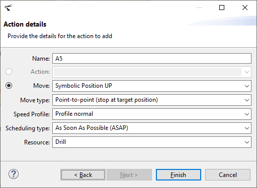
Adding a new action
-
Select Action from the Palette at the right side of the editor.
-
Left click somewhere in the green swim-lane of a peripheral. A popup window as the one above will show up.
-
Provide a name for the action.
-
Use the radio button to select the type of action you want to create. If the action is of type Move, then you must also specify if it is point-to-point (stop at target position) or on-the-fly (don’t stop at target position) and the speed profile to use.
-
Select the scheduling type - As soon as possible (ASAP) or As late as possible (ALAP)
-
Click Finish.
-
New action illustrates an example. In this case, the new action is A7.
Modifying the properties of an existing action
-
Select the action you would like to modify from the activity diagram.
-
Select the Properties tab in Eclipse. It is usually located below the diagram.
-
You should now have access to a menu that looks like the image below.
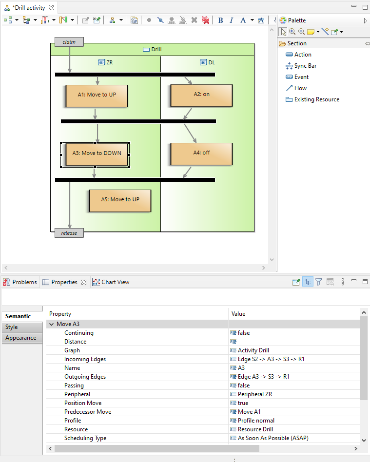
| You can use the Properties view to change the scheduling type of an action from ASAP to ALAP or vice versa. |
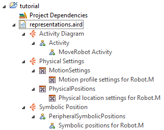
3.3. Location of Generated Graphs
The generated graphs are located inside its target element. By unfolding the element from the Model Explorer, the generated graphs will appear.
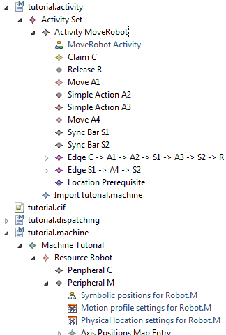
All the graphs can also be found under the “representations.aird” file.
3.4. Navigation among graphs
In graphical viewer, if one semantic element can be generated more than one graph, these graphs can be navigated. Navigation only happens when the semantic element is shown as a container/block in a source graph. Since there is no container concept in table, there is no navigation starting from a table view. Besides, navigations also request the target graphs have already been generated.
3.4.1. Navigate from activity diagram
A peripheral is represented as a write block in an activity diagram.
Some white blocks contain a small graph icon  at right bottom corner.
It means there are other graphs can be generated for the semantic element
of this block.
at right bottom corner.
It means there are other graphs can be generated for the semantic element
of this block.
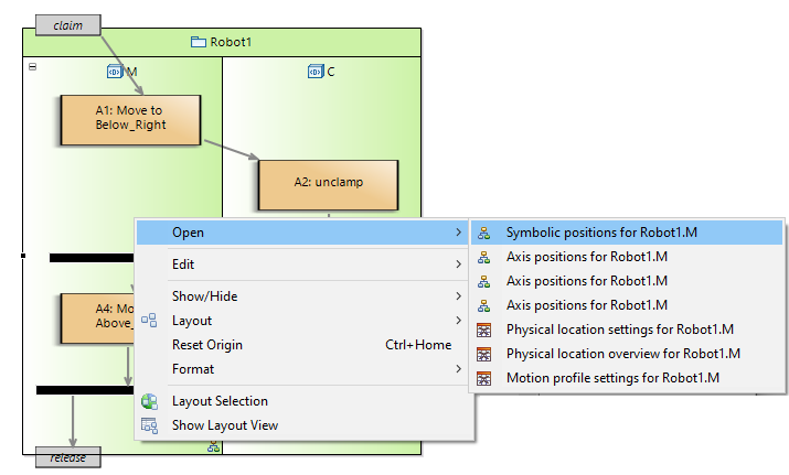
Right click on the write block, open with a desired graph. Movable peripherals can produce five types of graphs: axis position graph, symbolic position graph, motion profile settings table, physical location settings table and physical location overview table.
3.4.2. Navigate from axis position graph
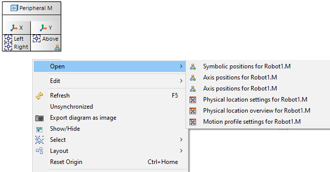
It is the same as navigation from activity diagram. Right click the container which has a small graph icon and open with a desired graph. From a axis position graph, it is possible to navigate to symbolic position graph, motion profile settings table, physical location settings table and physical location overview table.
3.4.3. Navigate from symbolic position graph
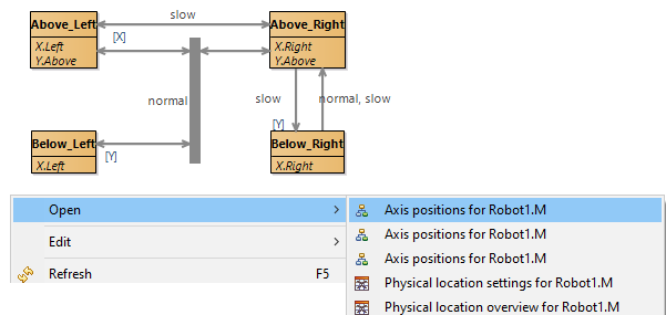
Right click the container which has a small graph icon and open with a desired graph. From a symbolic position graph, it is possible to navigate to axis position graph, motion profile settings table, physical location settings table and physical location overview table.
4. Schedule Activities
4.1. Scheduling & Configurations
| Scheduling an activity sequence requires a fully specified system. See section Logistics Specification for more information on creating this specification. |
Scheduling an activity sequence generates a Gantt chart that represents the system execution in time. Within an activity sequence one or more activities can be included. These activities will be scheduled as parallel as possible adhering to the claim/release strategy. If activities cannot be scheduled in parallel the order of this section is applied. An activity typically starts with claiming a Resource, hence this activity can only start if it predecessor activity has released this Resource.
Optionally an offset can be defined for an activity sequence. The scheduler will ensure that these activities will not be started before the offset time.
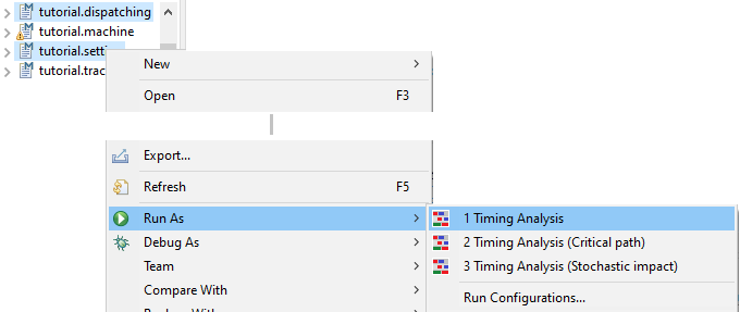
The easiest way to run a Timing Analysis is to select a dispatching file and a compatible setting file. Then right click and select Run As/Timing Analysis.
| Use <ctrl> <click> to select more than one item |
| You can explore the effect of different settings by combining a dispatching file with different setting files. |
For more advanced scheduling options you can use the Run Configurations window. Follow the above selection procedure but choose Run As - Run Configurations…, or use the dropdown from the green play button in the toolbar on top.
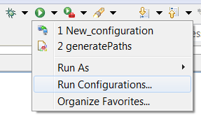
Available scheduling configurations show in the list on the left side of the Run Configurations window below the entry for Timing Analysis.
A new configuration can be created by using the New Launch Configuration button 
|
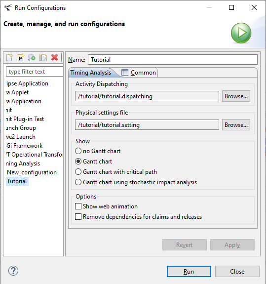
A Timing Analysis run configuration consist of the following elements:
-
Name Allows the user to identify the configuration for future usage.
-
Activity Dispatching Each configuration refers to one particular dispatching file. This is a required field.
-
Physical settings file The settings to be used to generate the schedule.
-
Show
-
no Gantt chart No Gantt chart is generated
-
Gantt chart A Gantt chart is generated and is shown on-screen. The timing of the Gantt chart is based on fixed timing settings and default values. The coloring is based on correspondence between Activities and Resources, see below for a more detailed explanation.
-
Gantt chart with critical path A critical path analysis of the schedule is made, based on fixed timing settings and default values, and is represented in a Gantt chart. The coloring is based on the outcome of the critical path analysis. See below for an explanation of the coloring scheme.
-
Gantt chart using stochastic impact analysis Based on fixed timing and default values a Gantt chart is generated. The coloring is based on the probability that a task will be on the critical path given the specified timing distributions. In order to determine this probability 200 samples are drawn. For each sample a schedule is determined and a critical path analysis is performed. See below for an explanation of the coloring scheme.
-
-
Options
-
Show web animation The scheduling produces skeleton files for Javascript/Paperscript based 2D animations. The default animation shows colored dots and by modifying the skeletons arbitrary animations can be produced. If the configuration also generates a Gantt chart an timing indicator is shown on the Gantt chart that is synchronized with the timing of the animation. The Javascript files are located at analysis/scheduled/animated.
-
Remove dependencies for claims and releases Before calculating the critical path the dependencies relating to claims and releases are cut short. As a result claims and releases are not included in the dependency graph and are thus removed from the critical path while preserving the net effective dependencies between actions. NB The claims and actions themselves are not removed from the schedule nor is the timing of the schedule influenced by this option.
-
4.2. Gantt Charts
The Gantt chart shows a resource on the Y-axis for every Peripheral which participates in the activity sequence. The X-axis shows the relative time in seconds. Each resource in the Gantt chart shows a low bar and a high bar:
| Low bar |
Represents the claiming of a Resource in the Machine by an Activity. This bar is replicated for all Peripherals in the claimed Resource. |
| High Bar |
Represents an action that is performed by a Peripheral. An action can be either a move or an atomic action. |
The arrows represent the dependencies between the tasks.
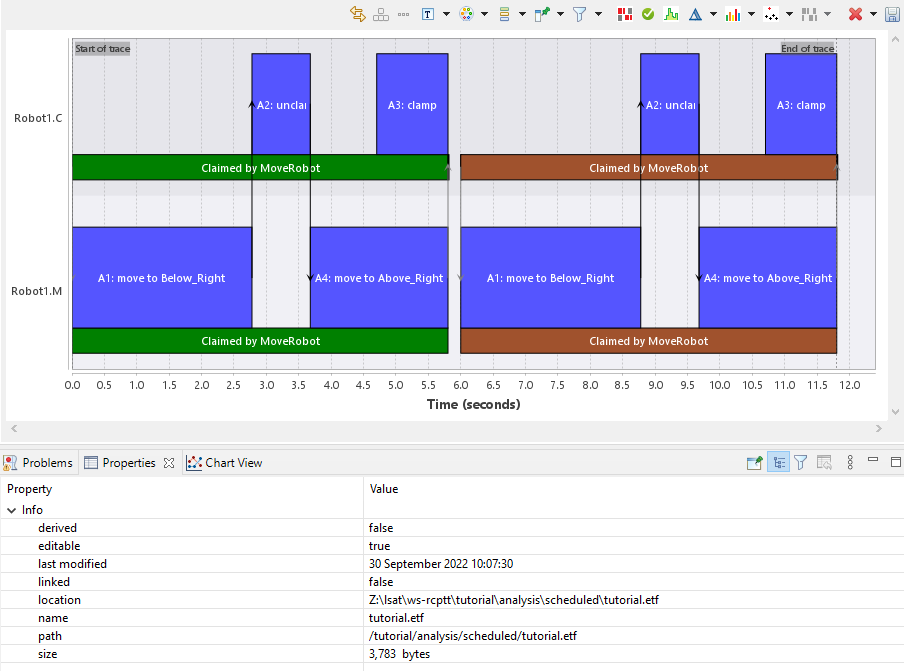
|
When a Gantt chart is generated, result files are stored in the project folder analysis/scheduled (i.e. a Gantt file <file>.etf). The file name of the etf file is derived from the file name of the dispatching file that is scheduled. The Gantt file is automatically opened in an editor showing the Gantt chart. |
| The Properties view shows detailed information about the selected bar. user attributes, trace points, scheduling phases and repeat steps will also be shown in the properties and can be used to filter the Gantt chart. |
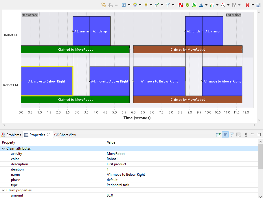
4.2.1. Gantt chart
In case of a Gantt chart without critical path analysis the color of the low bars represent the Activity that holds the claim. Additionally all actions, the high bars, of the same Resource are colored equally. The black arrows indicate the dependencies as specified in the Activity and the gray arrows indicate the dependencies between Activities as derived from the claim/release strategy.
If a resource is passively claimed by multiple activities then the properties show the activities that apply.
For passive claims the name shown is Claimed passively by …
Scheduling the actions in the activities
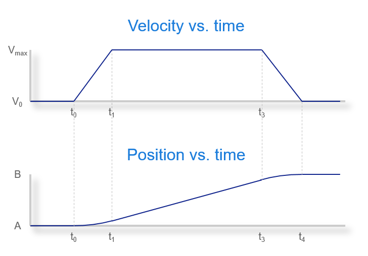
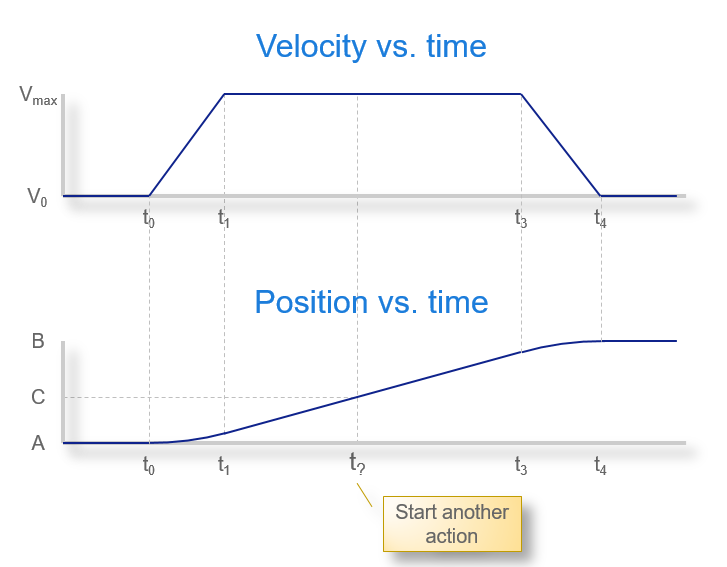
An action can be scheduled using two types of algorithms: As Soon As Possible (ASAP) or As Late As Possible (ALAP). The default algorithm for all actions is ASAP,
unless specified otherwise as described in Logistics Specification. As mentioned previously, resource claiming or releasing are always ASAP by design.
ASAP executes each action on a resource as soon as the resource is available, and all preceding actions have finished.
ALAP executes each action on a resource as late as possible. You can see the difference between the two schedules illustrated below.
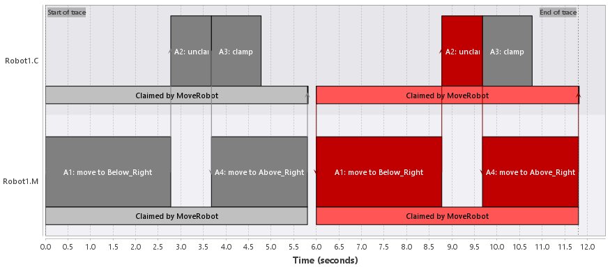
4.2.2. Gantt chart with critical path
In project management the critical path is defined as “the sequence of scheduled activities that determines the duration of the project.” The same applies for the calculated schedule as visualized in the Gantt chart.
When a critical path analysis has been performed the actions and dependencies are either colored red or grey. Red indicates an action or dependency is on the critical path of the schedule. The low bars can be dark red, light red or grey. Dark red indicates both claim and release are on the critical path. Light red indicates either claim or release, but not both, are on the critical path. Grey is used to indicate neither claim or release are on the critical path.
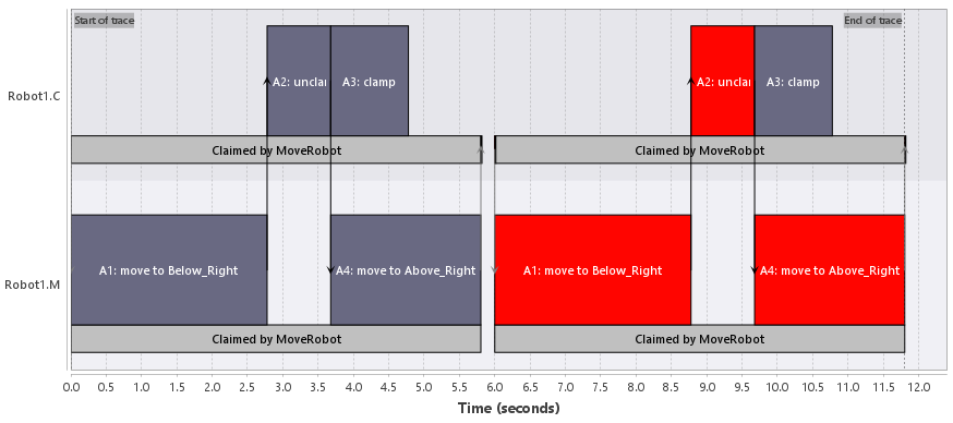
4.2.3. Gantt chart using stochastic impact analysis
The actions in the Gantt chart of the stochastic impact analysis are colored based on the probability that the action is on the critical path taking into account the specified timing distributions. A dark bluish grey indicates that the action will never be on the critical path, bright red indicates the action is always on the critical path. Intermediate colors are used to indicate intermediate probabilities. Tasks can be selected by using the mouse and the Properties window shows the property Critical that displays the probability that the selected task is on the critical path.
4.2.4. Filtering
By default the Gantt chart will hide all superfluous information. To show all information in the Gantt chart use the Eclipse TRACE4CPS toolbar to Clear all filters. Now all dependencies a drawn and also the dispatching offset is visualized.
| For more information about the possibilities in the ESI Trace viewer, see the TRACE user manual in the Help menu. |
5. Throughput per Resource Editor
The throughput per resource editor helps to identify where the specification can be optimized for throughput performance of the system.
As the specification is partitioned in multiple files (i.e. dispatching, settings, schedule, etc.) this makes it rather difficult to identify where the specification can be optimized for throughput. For this a new view has been designed which provides an overview of the most critical information with respect to throughput optimization for a specific activity dispatching sequence.
For each resource in the specification a tab page is available in the editor. The tab page shows an ordered table with all actions that are relevant for its resource. More information about the table content can be found in section The Resource Actions Table. The Outline view shows an overview of the throughput per resource and the throughput of the total activity dispatching sequence, for more information see section The Outline View.
5.1. Opening the Throughput per Resource Editor
The Throughput per Resource editor shows information for a specific activity dispatching sequence. For this reason the editor can be opened by means of the context menu of a particular dispatching file. The use of the context menu is needed as by default the Dispatching Editor is opened when double-clicking a dispatching file. To open the Throughput per Resource editor right-click a dispatching file in the Model Explorer view and select Open With → Throughput per Resource Editor from the context menu.
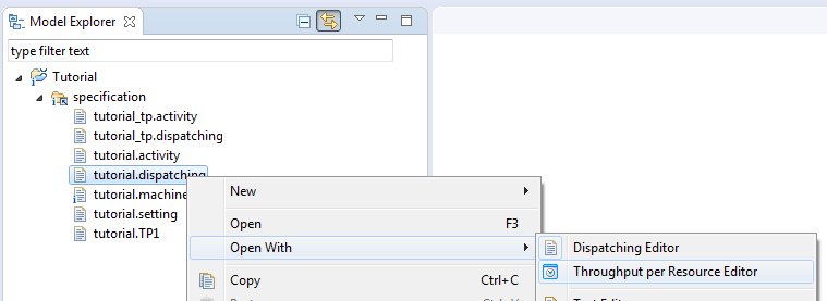
| Eclipse remembers the last editor used to open a file. When double-clicking the file this editor will be used again to open the file. The Open With context should be used to open the file using another editor. |
5.2. The Resource Actions Table
The resource actions table contains a row for every action in the activity dispatching sequence that is relevant for the resource. The rows are ordered as such that their actions are ordered in topological order w.r.t. the activity dispatching sequence. Topological ordering basically means that an action will never be listed before all actions required to be executed prior to the action. So this doesn’t guarantee that two succeeding actions in the table are executed in sequence as they might be executed in parallel. For more information on how the action sequence is determined please see section Calculating the Throughput per Resource.
In general a table cell will be gray when its information is not applicable for the action at that table row. When needed the data in the table either can be refreshed or reloaded.
Refreshing the data - by means of the  toolbar button - will update all data in the resource actions table and Outline view reflecting the current state of the editor including already made changes.
Reloading the data - by means of the  toolbar button - will discard all made changes and reload the specification models. This action can be used to reload changes in the specification which are made outside the Throughput per Resource editor.
| The Throughput per Resource editor will not detect added/deleted resources, axes and setpoints. When these are modified the Throughput per Resource editor needs to be closed and re-opened again. |
The table contains the following columns:
| Peripheral |
The fully qualified name (format <Resource Name>.<Peripheral Name>) of the peripheral performing the action. |
| Action |
The fully qualified name (format <Activity Name>.<Action Name>) of the action. |
| Name / From / Distance |
Either the name of the peripheral action, the start position or the distance of the move. |
| To |
The end position for the move (if applicable). |
| Settling |
The axes that require settling for the move. |
| Old <Axis> |
The start location per axis for the move. |
| New <Axis> |
The end location per axis for the move. An icon |
| Profile |
The motion profile name for the move.
The |
| <Setpoint> time |
For every setpoint, the minimum time needed to adjust the setpoint using its axis motion profiles. In other words, the time needed to adjust the setpoint conforming to its motion profile, not taking into account the adjustment of other setpoints, thus no stretching will be applied. |
| Time |
The time needed to perform the action. An icon |


| When editing: If the setting file contains a composed expression it will be replaced with the edited constant value. |
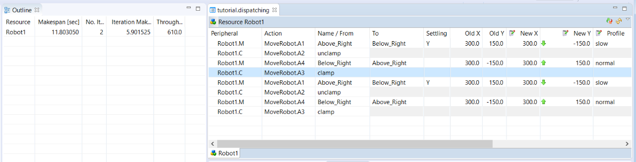
5.3. The Outline View
The image in the previous section also shows the Outline view. This view shows a table with an overview of the throughput per resource and - in the last row - the throughput for the total activity dispatching sequence. For more information on how the throughput is calculated for a resource, please see section Calculating the Throughput per Resource.
The table contains the following columns:
| Resource |
The resource for which the throughput is calculated. |
| Makespan |
The total time needed to perform all resource actions in the activity dispatching sequence. |
| No. Iterations |
The number of iterations for this resource in the activity dispatching sequence, for more information see section Specifying the number of iterations. |
| Iteration Makespan |
The total time needed to perform exactly 1 iteration in the activity dispatching sequence. |
| Throughput |
The theoretical maximum number of iterations per hour that this resource is capable of executing. |
5.4. Calculating the Throughput per Resource
This section provides some background information on what is meant by calculating the throughput per resource.
Though the systems throughput performance is determined by the full orchestration of all actions for all resources and peripherals in the system, sometimes it is good to know which resource is most critical in this orchestration. When calculating the throughput per resource the theoretical maximum throughput of the resource is calculated as if no actions of other resources are limiting its throughput, with the exemption of all actions in the 'entangled' section of an activity.
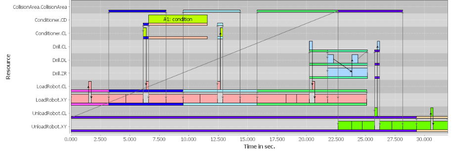
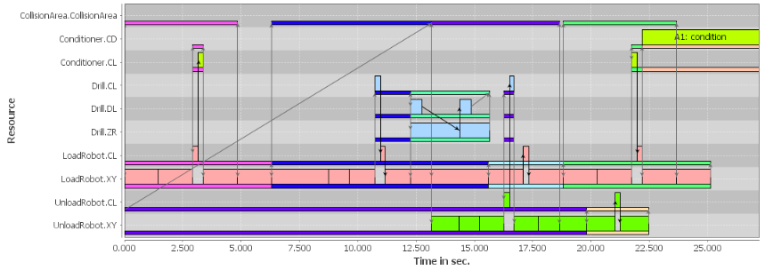
With the entangled section of an activity the section is meant in which multiple resources are working together in harmony, most likely to transfer a product from one location to another. Maybe this can be explained a bit easier by use of the following example. The figure below shows the schedule of an activity dispatching sequence with an overlay that illustrates the pre, post and entangled sections of an activity. The activity 'Robot1_GiveTo_Robot2' is repeated twice in the dispatching.
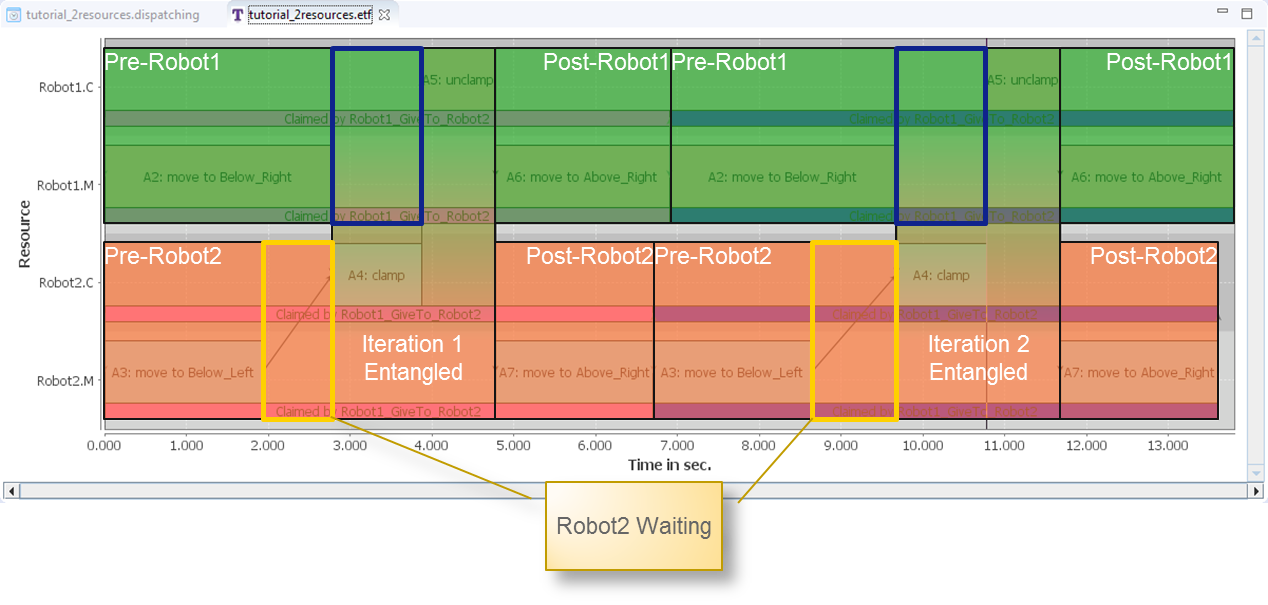
In the entangled section Robot2 first needs to clamp before Robot1 is allowed to unclamp. This causes a gap in the schedule of Robot1 as illustrated by the blue rectangles. As these gaps are within the entangled section, they are kept in the schedule when calculating the throughput for Robot1.
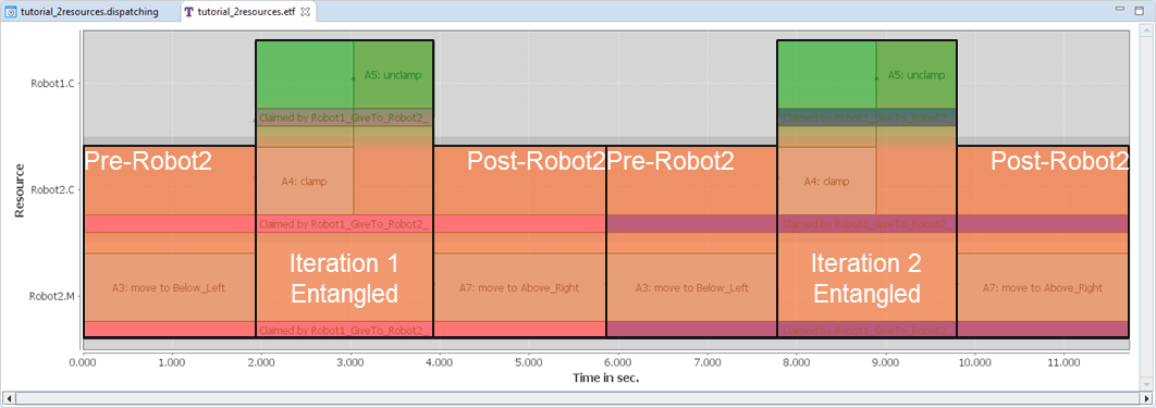
Additionally to gaps in the entangled section, Robot2 also has gaps in the schedule in its prepare section, as illustrated by the yellow rectangles in the schedule. These gaps are caused by Robot1 delaying Robot2. For calculating the throughput for Robot2 the pre and post sections of Robot1 will be omitted and a schedule will be used as illustrated in the following image.
6. Generating an Optimal Activity Dispatching Sequence
A supervisory controller modeled using CIF, see Create Supervisory Controller Specification, captures all possible activity dispatching sequences. Given such a specification, an optimal activity dispatching sequence can be computed. We distinguish between two situations:
-
Optimal continuous processing of products In the first case, the supervisory controller specifies all possible activity sequences to establish a continuous product flow. The supervisor should have cycles, which represent repeatable activity sequences, modeling the continuous processing of products. An optimal activity dispatching sequence can be generated, that contains a repeatable activity sequence achieving the maximum throughput, as well as the transient activity sequence to get to this steady-state repeatable activity sequence from the initial system state.
-
Optimal processing a batch of products In the second case, the supervisory controller specifies all possible product flows for a batch of products. The supervisor should not have any cycle. It is assumed that any path to a final state without enabled edges means that the product flow successfully completed. An optimal activity dispatching sequence can be generated, that achieves the minimum makespan, i.e., the fastest way to execute all required activities and reach a final state.
6.1. Generating a Dispatching File for Maximum Throughput
Target element: an activity specification
Right click on a target element, select Generate Dispatching File (throughput) to generate an activity dispatching sequence with maximum throughput.
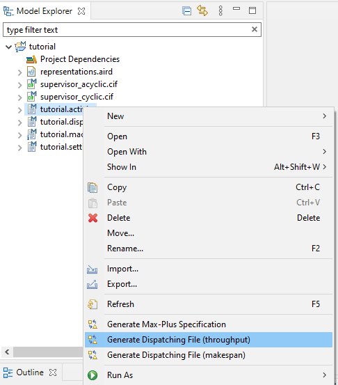
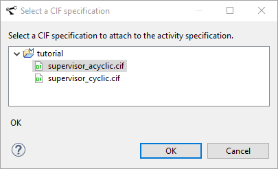
Select a relevant CIF specification file.
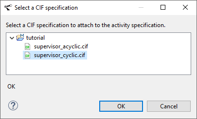
In this example, we use the following CIF specification.
controllable MoveRobot;

supervisor Tutorial:

  location l0:
    initial;
    edge MoveRobot goto l1;

  location l1:
    edge MoveRobot goto l0;

end
Click 'OK' to start running the throughput analysis.
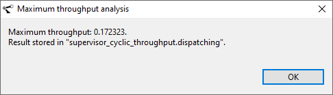
Once the analysis is finished, the computed throughput value is reported.
The dispatching file containing the optimal activity dispatching sequence is generated in the result folder.
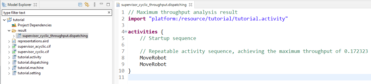
The first part of the dispatching file specifies the activity sequence that is needed to reach the steady state of the system. In the steady state, the same repeatable activity sequence can continuously be executed. In our example, this steady state is immediately reached. The throughput is defined as the number of activities that are executed, divided by the total execution time of the cycle. In our example, the throughput is 2 activities / 11.606 sec = 0.1723 activities per second.
This can visually be shown in the following corresponding Gantt chart.
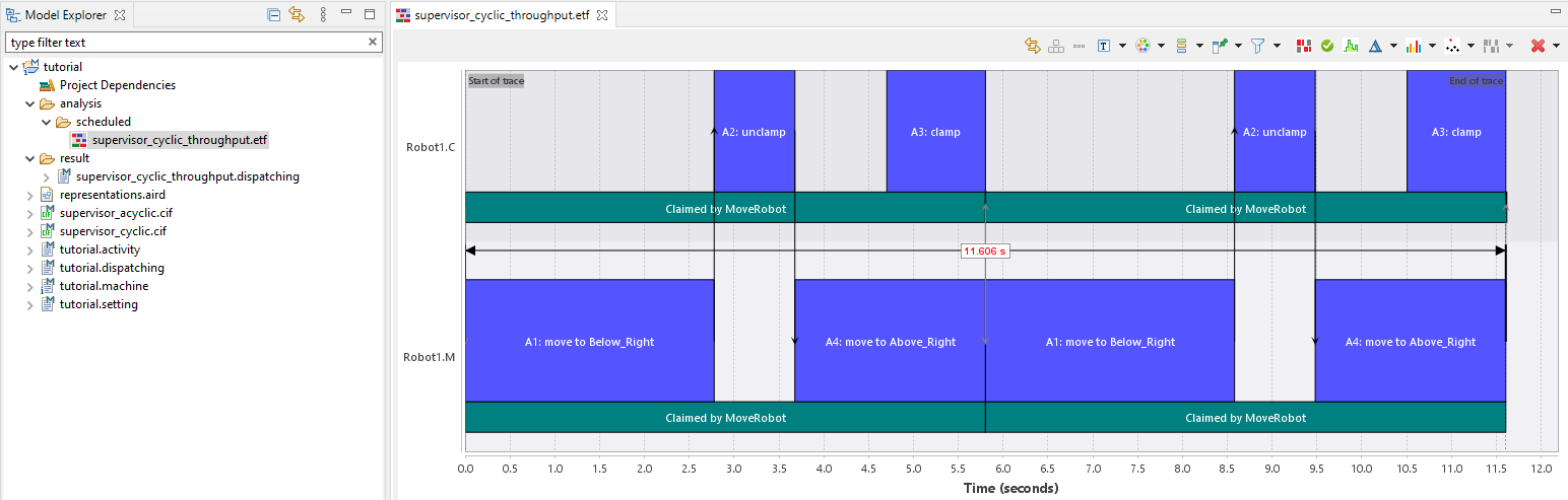
| To scheduled the generated activity dispatching sequence in the form of a Gantt chart, see section Schedule Activities. |
|
To calculate the maximum throughput, the CIF file must contain a cycle. 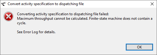
|
6.2. Generating a Dispatching File for Minimum Makespan
Target element: an activity specification
Right click on a target element, select Generate Dispatching File (makespan) to generate an activity dispatching sequence with minimum makespan.

Select a relevant CIF specification file.
In this example, we use the following CIF specification.
controllable MoveRobot;

supervisor tutorial:

    location l0:
        initial;
        edge MoveRobot goto l1;
    location l1:
        edge MoveRobot goto l2;
    location l2;
end
Click 'OK' to start running the makespan analysis.
Once the analysis is finished, the computed makespan value is reported, which is the total execution time of the activity sequence.
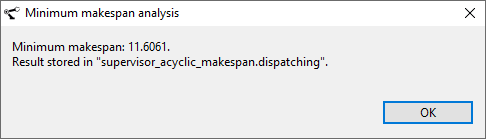
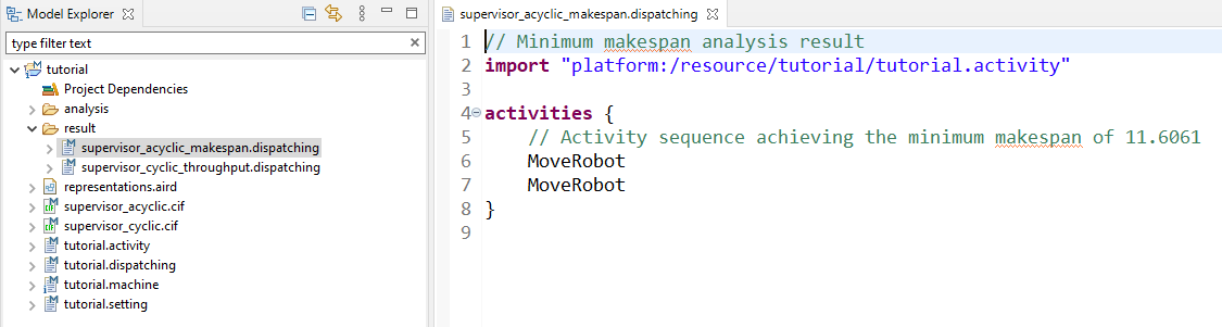
The dispatching file showing the optimal activity dispatching sequence is generated in the result folder.
|
To calculate the minimum makespan, the CIF file must not contain a cycle. 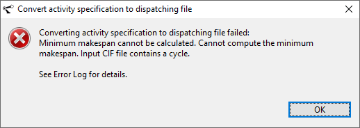
|
6.3. Viewing Makespan/Throughput Values
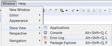
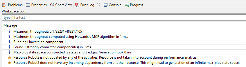
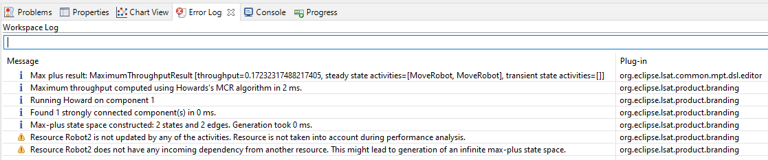
The minimum makespan/maximum throughput, as well as some details about the algorithm execution, can be seen in the Error Log view. The Error Log view can be opened by clicking Window in the toolbar on top and Show View → Error Log.
|
An infinite state space can be generated during the throughput analysis, if there are multiple resources that can execute actions without ever synchronizing. A warning is generated if a resource is nowhere used in the analysis, or if it is never synchronized with another resource. To prevent a never terminating analysis, these problems should be resolved in the specification. |
7. Conformance Check
Conformance checking functionality is used to check whether traces from log files are able to be projected to a certain dispatching.
7.1. Add Trace Point
Before conducting a conformance check, trace points are supposed to be added to activity specifications. Trace points, logged in trace log files, are used to identify the starting and end points of an event. An example of log file is given below. Each line in a log file contains all the information of time and a trace point.
By default, log files with an extension trace are supported for conformance checking.
A trace file is line based where each line starts with an instant in UTC (i.e. parsed using DateTimeFormatter.ISO_INSTANT), followed by comma-space and then the trace point.
|
2011-12-03T07:15:30.454994Z, TP-0001
2011-12-03T07:35:15.454894Z, TP-0002
2011-12-03T07:35:15.455168Z, TP-0005
2011-12-03T07:35:15.455172Z, TP-0006
2011-12-03T07:35:15.455429Z, TP-0007
2011-12-03T07:35:15.455434Z, TP-0008
2011-12-03T07:35:15.455588Z, TP-0009
2011-12-03T07:35:15.455591Z, TP-0011
2011-12-03T07:35:15.455797Z, TP-0010
2011-12-03T07:35:15.455805Z, TP-0012
2011-12-03T07:35:15.456519Z, TP-0003
2011-12-03T07:35:15.456716Z, TP-0004
In the first line, “TP-0001” is the string identifying the trace point in principle which is unique throughout the entire log files.
Additionally, there must be a trace point specification, which maps a trace point to either a starting or an end point of a known action. For instance, TP-0001 maps to start claiming Robot. In order to perform conformance check, trace points are supposed to be added to its related activity specification surrounding an action definition.
import "tutorial.machine"

activity MoveRobot {
  prerequisites {
    Robot1.M at Above_Right
  }
  actions {
    C: ["TP-0001"] claim Robot1 ["TP-0002"] (1)
    R: ["TP-0003"] release Robot1 ["TP-0004"]
    A1: ["TP-0005"] move Robot1.M to Below_Right with speed profile slow ["TP-0006"]
    A2: ["TP-0007"] Robot1.C.unclamp ["TP-0008"]
    A3: ["TP-0009"] Robot1.C.clamp ["TP-0010"]
    A4: ["TP-0011"] move Robot1.M to Above_Right with speed profile normal ["TP-0012"]
  }
  action flow{
    C -> A1 -> A2 -> |S1 -> A3 -> |S2 -> R
                     |S1 -> A4 -> |S2
  }
}
| 1 | ["TP-0001"] and ["TP-0002"] represent starting and end points for claiming a Robot. |
7.2. Conduct Conformance Check
After adding all the trace points to an activity specification, conformance check can be applied upon a dispatching file.
| Dispatching offset is not supported for conformance check currently. |
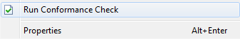
Right click on a dispatching file and select Run Conformance Check.
Note that in order to obtain a successful conformance check based on the above activity file, the dispatching file look like:
import "tutorial_tp.activity"

activities {
  MoveRobot ("First product")
}
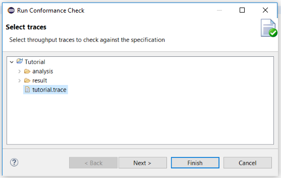
Select trace files to run the conformance check, and Next.
There are several configurations for conformance check.
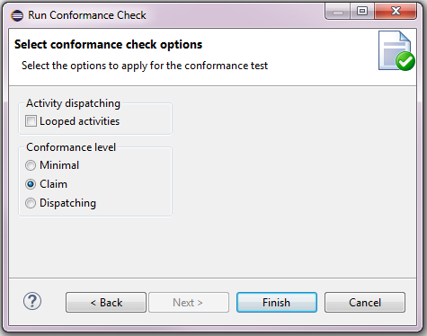
| Activity dispatching |
Selected, if it activity dispatching occurs multiple times in log files. |
| Conformance level |
There are three levels for conformance check. |
Set conformance check options and Finish. The conformance check will be executed.
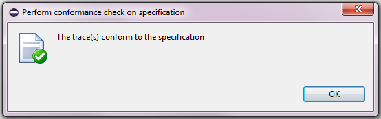
After the progress is completed, a pop-up will appear to show whether or not it passes the conformance check.
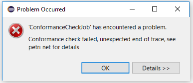
If a conformance check fails, a petrinet file will be generated under the folder analysis/conformance. It is used to diagnose conformance check failure.
In order to open a graphical view of a Petri Net, a new viewpoint needs to be added to the project.
| If the Analysis viewpoint is not visible, please restart your Eclipse using . |
Navigate to a Petri Net model element to open an existing graphical view or right click it to create a new one.
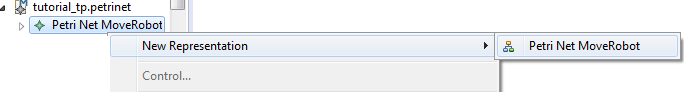
A graphical view is opened.
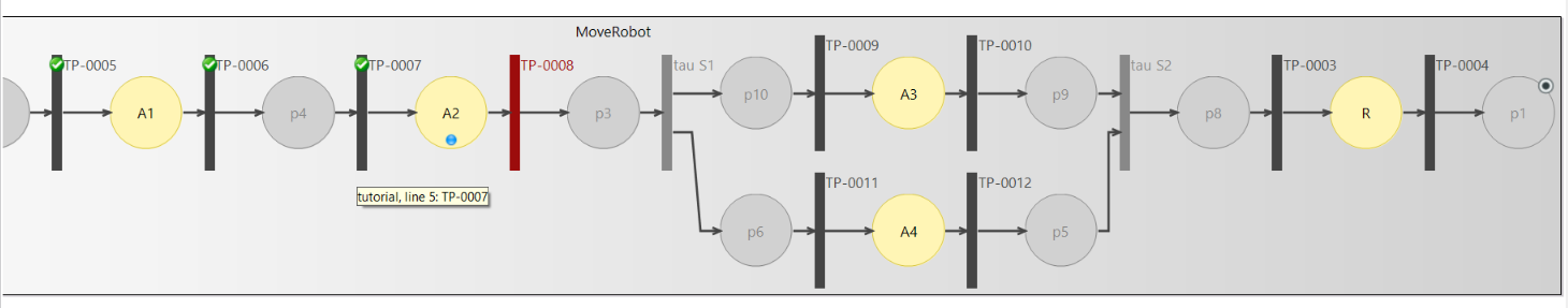
The Petri Net shows how the trace lines are projected upon it.
Black Bar - it represents a trace point transition. A green arrow on top indicates this trace point transition has been passed.
Gray Bar - it represents a transition doesn’t require a trace point check.
Red Bar - it represents an armed transition with a certain trace point is expected. Usually, it is a place where an error occur.
Yellow Circle - it represents an action as a place.
Gray Circle - it is a place to connect two transitions, if there is no action in between.
Blue Token - it indicates where the conformance check stops.
7.3. Filter Trace Point
Filtering out irrelevant trace points in log files is not required for conformance check. However, it helps to reconstruct activities manually, especially when the amount of irrelevant trace points is much more than the relevant ones. Before filtering, activity specification should be inserted with trace points.
Right click log files and select Filter traces.
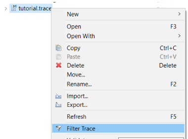
Select Activity elements which contain all the relevant trace points and continue with OK.
After filtering, selected log files will only keep the trace points which are used in activities.
8. Generate Max-Plus Specification
The timing behavior of an activity execution is characterized by two elements, which are:
| synchronization |
waiting for incoming claims, releases, or actions to finish |
| delay |
action duration (specified either directly in the settings file, or derived from a motion specification) |
A max-plus matrix can be used to concisely capture this timing behavior. The matrix describes the longest path between each resource claim and release. Computing the total execution time of an activity sequence can be done by multiplying the corresponding max-plus matrices.
The max-plus specification also contains the supervisory controller described by CIF. Given all possible activity sequences and the corresponding max-plus matrices, the worst-case and best-case throughput and makespan can be computed.
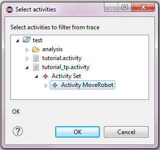
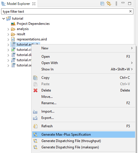
To generate a max-plus specification, click on the activity file and select "Generate Max-Plus Specification".
Next, select the respective CIF file. If the CIF file contains cycles, the minimum/maximum throughput can be computed. If the CIF file does not contain cycles, the minimum/maximum throughput can be computed.
Modify the CIF file as it is shown below in order to include a cycle.
controllable MoveRobot; (1)

supervisor Tutorial: (2)

  location l0:
    initial; (3)
    edge MoveRobot goto l1; (4)

  location l1:
    edge MoveRobot goto l0;

end
Now, we are ready to generate the activity dispatching sequence ensuring the maximum throughput.
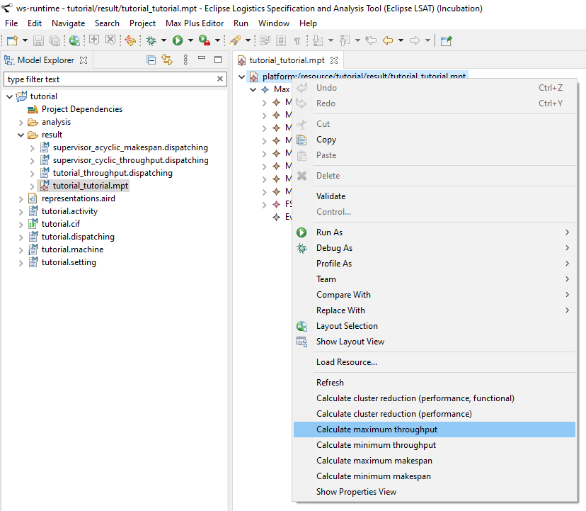
The result of the computation is shown in the Error Log, including some additional details about the computation times of the steps.
|
The max-plus specification is used mostly for experimental features, including for example partial-order reduction. Computing the maximum throughput or minimum makespan can also done without first computing the max-plus specification, as described in Generating an Optimal Activity Dispatching Sequence. |
9. Generate GraphML from CIF specification
Eclipse LSAT™ also gives you the opportunity to generate a GraphML diagram from a CIF specification. This feature allows the user to verifying the correctness of the CIF specification.
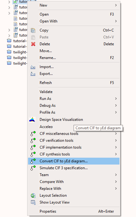
To do so, execute the following steps:
-
Right click on the desired file containing the CIF specification.
-
Select Convert CIF to yEd diagram.. as shown in the figure above.
-
Select your desired output from the available radio buttons: error, warning, normal or debug.
-
Press OK.
-
Two new files should be generated:
-
(name of your cif file).model.graphml
-
(name of your cif file).relations.graphml
-
For the official documentation on the CIF to yEd transformer, click here.
10. Twilight Manufacturing System: a showcase
The first step for using Eclipse LSAT™ in industry is to decompose the manufacturing system into a plant by defining resources, peripherals, actions and the respective activities ordering.
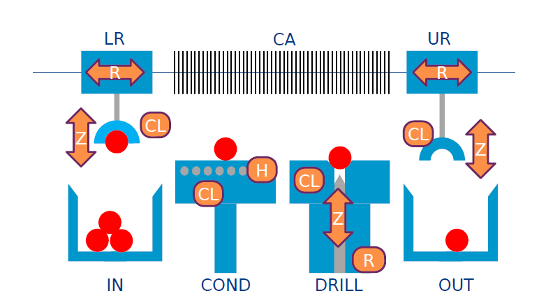
In this section, we introduce the Twilight System to show a use case of Eclipse LSAT™ in industry. Twilight refers to a simplification version of a wafer handling sub-system used at ASML. This system is presented in the figure:
The components of a system are described by resources. Each resource consists of one or many peripherals.
The behavior of the system is modeled on three levels:
-
Actions: executed by peripherals.
-
Activities: used to describe scenarios of end-to-end deterministic behavior. An activity consists of a set of actions and dependencies among these actions.
-
Activity sequences: used to describe orderings of activities.
Within the respective system, the Resources are Collision Area (CA), Load Robot (LR), Conditioner (COND). Each resource contains usually more than one peripherals, for example resource LR is composed of three peripherals: the R and Z motors and the CL clamp. The motors allow LR to move within a certain area, whereas the CL clamp allows it to grasp/release a product.
The actions are:
-
Claim and Release resources;
-
Unclamp, Clamp, Moves.
The basic activities are: Condition and Drill, whereas those related to the moving are: LR_PickFromInput, LR_PickFromCond, LR_PickFromDrill, LR_PutOnCond, LR_PutOnDrill UR_PickFromCond, UR_PickFromDrill, UR_PutOnCond, UR_PutOnDrill, UR_PutOnOutput.
The name of the activities can be easily connected to the respective meaning based on figure:
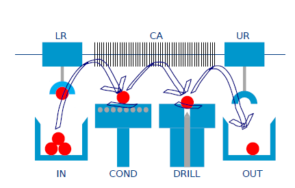
Based on the dispatching file which specifies the ordering of activities, a feasible schedule can be generated, which meets the constraints related to the resources and the synchronization/delays.
As explained in Generating an Optimal Activity Dispatching Sequence, this schedule can be optimized in terms of throughput/makespan based on the information included in the CIF file.
The figure above shows the ordering of the activities for an optimal throughput.
For an extensive explanation regarding the theory and the examples based on Eclipse LSAT™, please refer to:
11. Release Notes
The release notes of the Eclipse Logistics Specification and Analysis Tool (Eclipse LSAT™) are listed below, in reverse chronological order.
11.1. Eclipse LSAT™ v0.3 (2024-02-15)
This release contains bugfixes, improvements and new features. For a complete overview of issues that are part of this release, please see the milestone v0.3 issue list. The highlights for this release are:
-
Parameterized events
To avoid duplicate activities, Eclipse LSAT™ already allowed pools of resources and parametrized activities. Parameterization is added for events to avoid activity duplication if events are used for synchronization.
-
Eclipse TRACE4CPS v0.1 → Eclipse TRACE4CPS v0.2
11.2. Eclipse LSAT™ v0.2 (2023-02-07)
This release contains bugfixes, improvements and new features. For a complete overview of issues that are part of this release, please see the milestone v0.2 issue list. The highlights for this release are:
-
Add support for passive claims in LSAT (issue #38)
A resource can be passively claimed to ensure that no actions are performed by any of its peripherals until the resource is released again. If more activities claim a resource passively, they potentially can run in parallel.
11.3. Eclipse LSAT™ v0.1 (2022-11-01)
This release contains the Eclipse LSAT™ initial contribution. This version is a port of ESI LSAT v2.0.1 that is prepared for its release to the Eclipse foundation, including:
-
Eclipse Neon → Eclipse 2020-06
-
ESI TRACE v0.63 → Eclipse TRACE4CPS v0.1
-
TU/e CIF3 → Eclipse ESCET v0.1
-
Modular setting files
-
Expression language
-
Resource pools; more concise specifications
-
User-defined attributes in dispatching file e.g., for product tracking
-
Multiple phases in dispatching file e.g., set-up, steady-flow and tear-down
-
Dependencies between activities
-
Motion profiles: support for rotational movements
-
APIs for integration of motion libraries (JSON and/or Java)