TRACE Little's-law-based analysis

NOTE: Analysis is applied to the current filtered view

Little's law (see, e.g., here) stems from queueing theory and relates throughput, latency and work in progress (wip). The TRACE tool supports the creation of continuous signals for these three properties from the discrete claims and or events in the trace. The resulting signal is added to the view, and can be removed by the "clear filters or extensions" menu (). The Little's-law menu () has four items, explained below.

Event-based throughput

This analysis computes the continuous throughput signal based on events. It has four parameters:

• Window width (in seconds): this parameter determines the width of the sliding window that is used to convolute the instantaneous throughput signal. For a window width of t, the resulting signal gives the average over the last t time units. If t=0 then the resulting signal is the instantaneous throughput.
• Value scale: this parameter, a time unit, determines the scale of the signal range.
• Event type: this parameter is the first part of the event filter and determines which event types (start event of a claim, end event of a claim, or any event) to use for the throughput computation.
• Attribute filter: this parameter is the second part of the event filter and determines which events to include for the throughput computation.

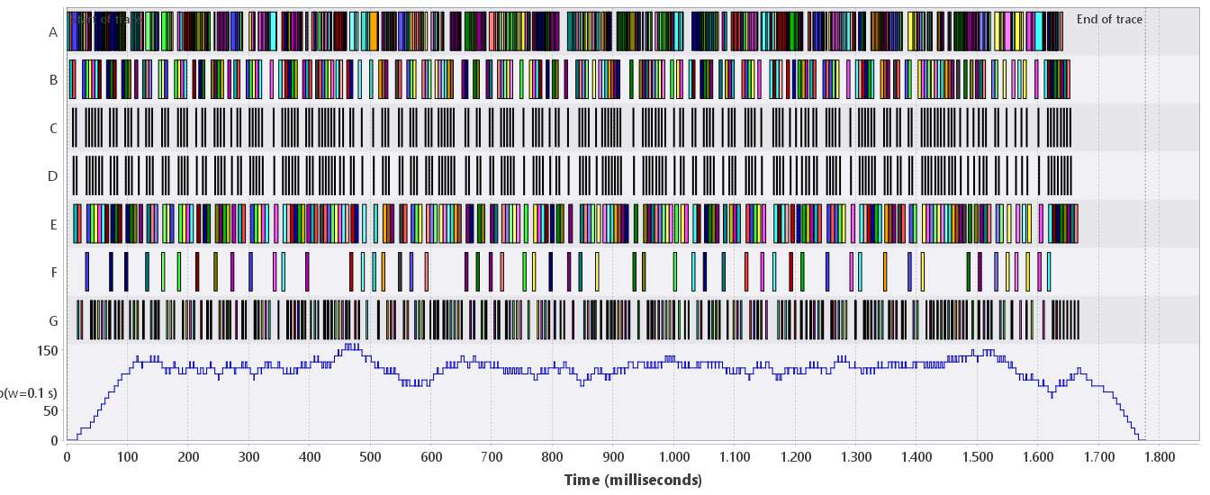
Figure 1 shows an event-based throughput signal for the running example. The window width is set to 0.1 seconds, the value scale is seconds (i.e., the throughput per second is computed), and the event filter is set to end events with name E (start and end events of claims have the same attributes as the parent claim). The throughput, a continuous signal, is added to the trace in a separate section (here at the bottom). The range of the signal gives the number of objects that are processed per second. Note that we do not use task G because it can be preempted, resulting in multiple end events per data object that is processed.

Identifier-based throughput

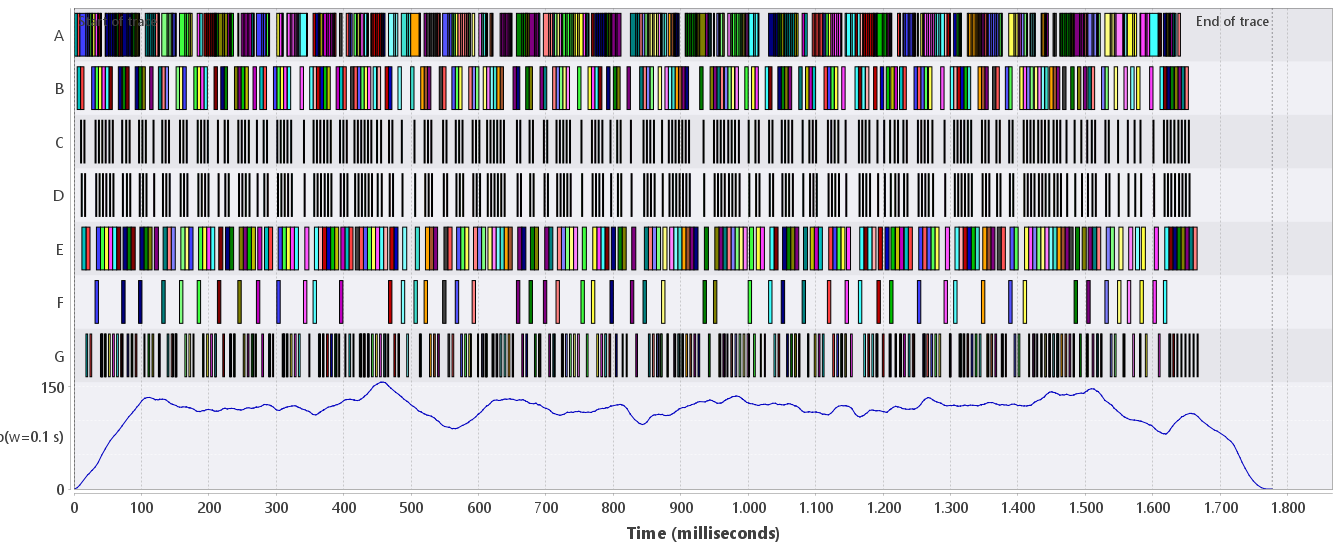
The identifier-based throughput analysis also has the window and value scale parameters. Instead of specifying a filter to include events for the throughput computation, a grouping attribute is used. All claims and events with the same value for that attribute are grouped and the analysis assumes that these all are involved by the processing of a single object. The earliest and latest time stamps in the group of claims and events are used to construct the throughput signal. It therefore usually gives a smoother graph than the event-based throughput. In the running example we can use the "id" attribute for grouping; see Figure 2. Here we have computed the identifier-based throughput in seconds with a sliding window of 0.1 s. It is similar to the graph in Figure 1, but smoother.

Identifier-based wip

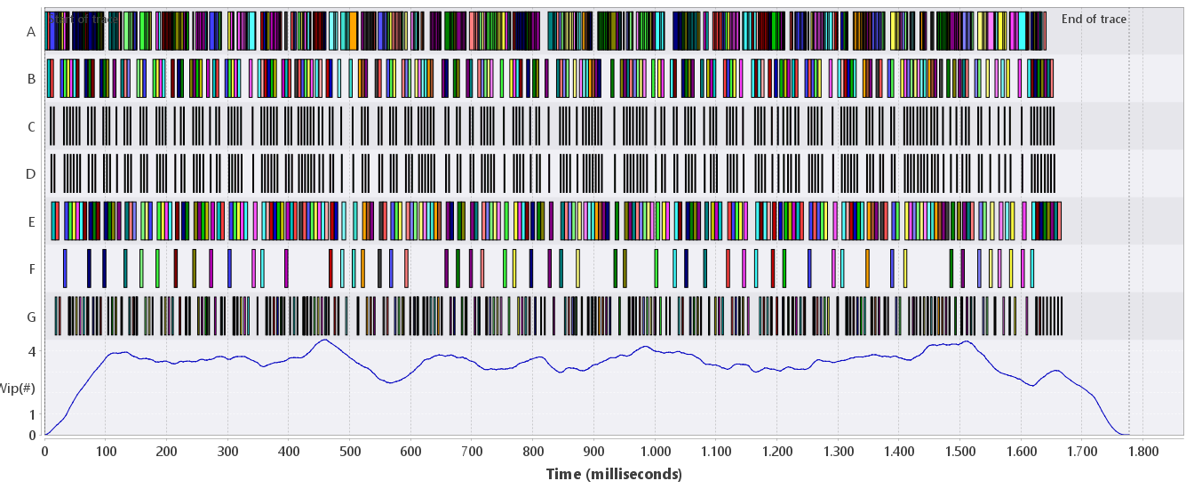
The wip analysis only needs the window width and the grouping attribute. It computes a signal that gives the number of objects that are being processed at the given time. Figure 3 gives an example using the "id" attribute for grouping and with a sliding window of 0.1 s.

Identifier-based latency

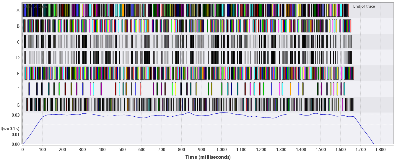
The latency analysis has the same parameters as the identifier-based throughput analysis. The latency signal is computed by applying Little's law to the throughput and wip signals. Figure 4 shows the latency signal in seconds with a window width of 0.1 seconds and grouping by the "id" attribute. The latency is around 30 milliseconds. Figure 2 shows that the throughput is about 120 frames/second, and Figure 3 shows that the wip approximately 3.5. Little's law informally states that wip = throughput * latency, which in our case approximately means that 3.5 ≈ 120 * 0.03 which indeed is approximatly correct.

The four type of signals described above are mathematically well-defined. It is, however, out of scope of this manual to explain those details here. A publication is forthcoming that covers all the math [5].