TRACE Visualisation

Opening a TRACE view

TRACE files (.etf files according to the format specified here) can be viewed by double-clicking them in the Project Explorer view. Multiple TRACE files can be opened in the same view by selecting them in the Project Explorer view, and then right-clicking the selection. In the context menu then select the "Open as TRACE view" item. Both ways of opening TRACE files result in a Gantt-chart view in the IDE.

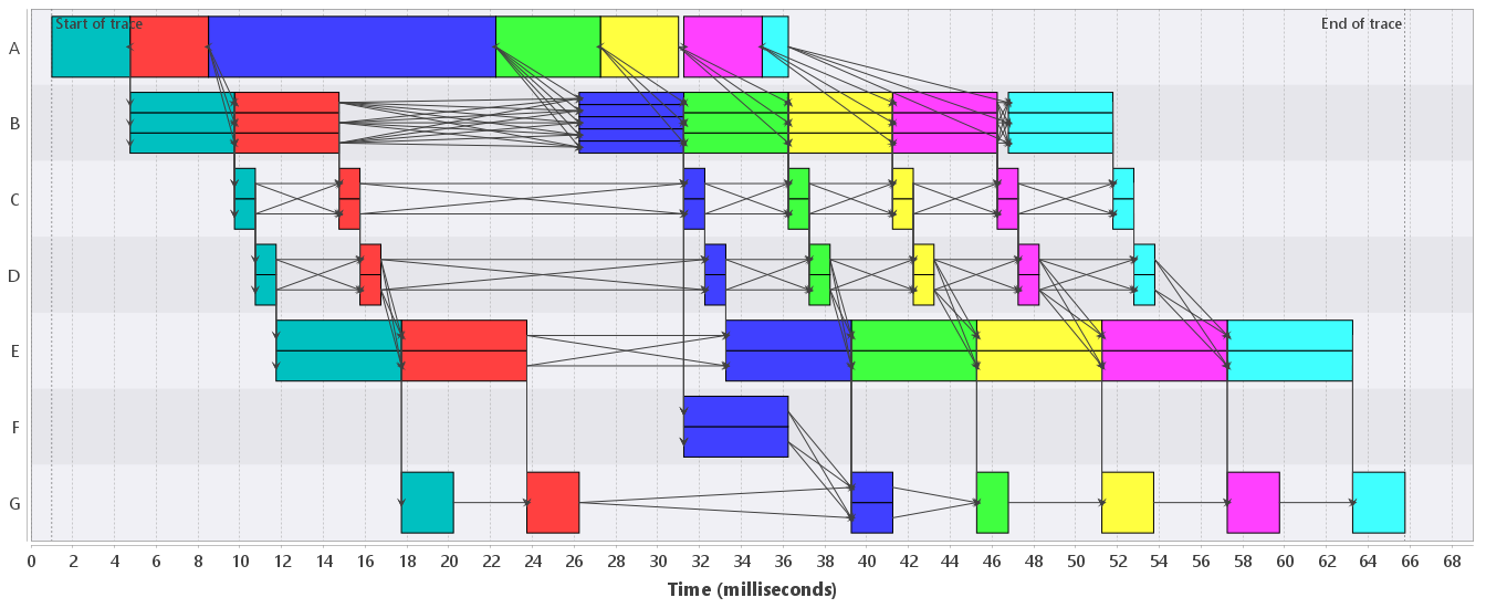
All TRACE entities (claims, events, signals, time-series and dependencies) are visualized in a chart with on the horizontal axis the time, and on the vertical axis a number of labeled sections. A single section contains a set of claims, a set of events, a single signal or a time-series. The grouping configuration (see below) determines how the claims and events are distributed over sections. The example in Figure 1 shows a part of a trace with claims and dependencies between claims. (It is a view on the "model-bf.etf" trace of the running example).

Basic viewing actions

Zooming and panning

Panning is done by Alt-down and dragging the chart.

Scrolling can be done as follows:

• Mouse wheel:
  • Scrolls on the horizontal axis (time) if no vertical scrollbar is present.
  • Scrolls on the vertical axis if a vertical scrollbar is present.
• The arrows on the scroll bars can be used for scrolling in smaller steps.

Zooming can be done in various ways:

• Right-click the chart: The context menu has several items to zoom one or both of the axes.
• Ctrl-down and mouse wheel zooms the horizontal axis in or out.
• Shft-Ctrl-down and mouse wheel zooms the vertical axis in or out.
• Area selection in the chart using the mouse zooms to that selection.
• A mouse dragging gesture to the left zooms out fully on both axes.

Selection and tooltips

Selection is supported for all concepts: claims, events, dependencies signals and time-series. The Eclipse Properties view shows the properties of the selected item. The selected item is shown with a yellow border. Tool tips are also supported for all five concepts. Sometimes it is unclear which points can be selected in a signal. Therefore, these points can be explicitly shown (see below).

Measurement tool

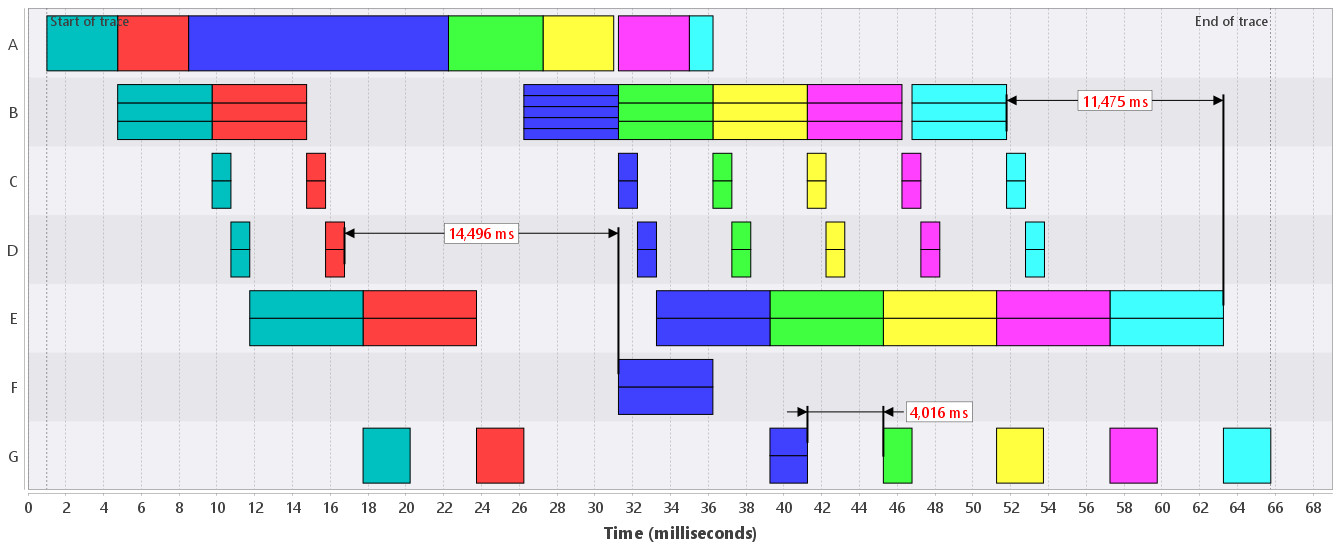
The measurement functionality can be used to measure the time between claims, events, signal and time-series segments. By hovering over such an entity, a vertical marker is shown. By a left-click of the mouse with Alt-down, a marker is set. Setting a second marker adds an annotation to the chart with the distance between the markers. Multiple annotations can be defined, see Figure 2. An annotation can be selected by clicking the label, and it can be deleted by pressing the delete key. Note that the annotation label can be dragged vertically.

Configuring the view

The view can be configured via a number of menus on the top right of the view part in the UI:

• switches between the activity and resource views
• toggles alphabetic sorting of trace parts
• opens a dialog to manually reorder chart rows
• switches between FULL and NONE scaling of the claims (only in activity view)
• opens font size settings for the chart
• toggles whether signal markers are shown
• selects the describing attributes for events, dependencies, claims, resources, signals and time-series
• selects the coloring attributes for events, claims, dependencies, and time-series
• selects the grouping attributes for events and claims (only in activity view)
• completely hides parts of the trace
• configures filters
• clears filters or extensions
• persists the current view

Each of these functionalities is explained below. Next to these items in the menu bar, there are other items that trigger analysis methods. These are explained in other sections.

Activity vs resource view:

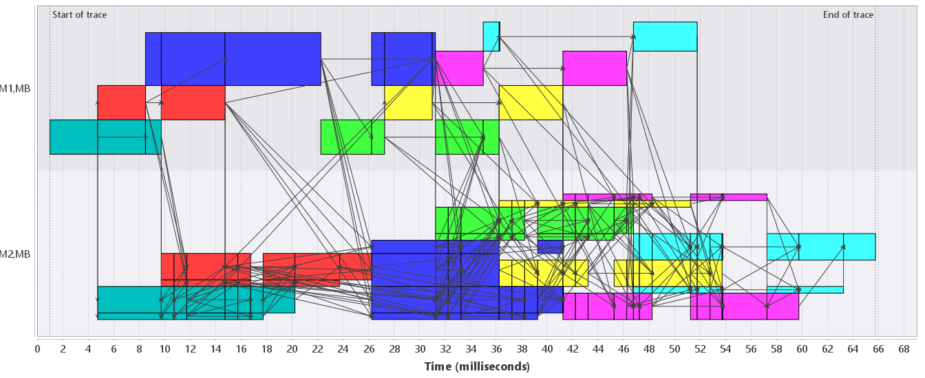
The distinction between activity and resource view is only about claims. In the resource view, the grouping is done according to the resource of a claim. I.e., all claims that use the same resource are in the same section. Furthermore, the scaling of each claim in the swimlane (i.e., its offset and height) is done according to the claimed amount and offset of the claim. In the activity view, the grouping of the claims is done according to the grouping attributes that can be defined by the user (see below). Figures 1 and 2 show the activity view, and Figure 3 shows the resource view (note that Figure 2 only shows the memory resources).

Alphabetic sorting:

Sort the trace parts (resources, signals, etc.) either alphabetically, or by the order in which they were specified in the .etf file. In the second case the resources are ordered by the start time of the first activity of each resource.

Manual row reordering:

Use this action to manually change the order of visible chart rows. The dialog shows the current rows and supports drag-and-drop reordering. After pressing OK, the order is applied to the chart and saved in the view configuration. If alphabetic sorting is enabled, manual ordering is not used.

Scaling of claims:

In the activity view the user can choose whether the scaling of claims is NONE or FULL. The former is the default value as it is more efficient than the FULL option. The difference between the options shows if there are claims in the same section that have an overlap in their time domain. With the NONE option, the claims are just drawn on top of eachother, which may hamper detailed inspection. With the FULL option, overlapping claims are stacked to fill the swimlane. In that way, overlap is made explicit, but the efficiency of the visualization may suffer.

Font size dialog:

The font dialog controls the chart text size (axis labels, section labels and other chart text). It supports two modes:

• Global mode: one font size for all TRACE views.
• Chart-specific mode: font size is stored in the current .view configuration file.

The dialog shows the size in pixels and applies a live preview while changing values. Use Reset to default to restore the default chart font size.

Signal markers:

The user can toggle the visualization of signal markers. There is a marked point in the signal for every polynomial fragment in the signal. Selecting such a point shows the properties of the fragment in the properties view.

Description:

This menu lets the user select the attributes that are used, e.g., for tooltips and section labels. The selected attributes have the following effects for the different trace parts:

• Events: The describing attributes are used for the tooltip and section label.
• Dependencies: The describing attributes are used for the tooltip.
• Claims: The describing attributes are used for the tooltip and section label. Furthermore, the checkbox show claim descriptions can be used to (de)activate labels based on the describing attributes inside the claims (if there is enough space to render the label).
• Resources: The describing attributes are used for the section label if in resource view.
• Signals: The describing attributes are used for the tooltip and section label.
• Time-series: The describing attributes are used for the section label.

Coloring:

The user can specify a subset of attributes for coloring claims, events and dependencies. These attributes are used to compute a coloring partition, i.e., a partition of the claims, events or dependencies into a set of disjoint cells such that all elements of a cell have the same attributes and values. All elements in a cell will have the same color. The current TRACE palette has approximately 40 colors, and each cell of the coloring partition is mapped onto this palette. In the figures above, we have used the "id" attribute for coloring.

There is also the option to explicitly specify the color of a claim, event or dependency. This is done by assigning an attribute named "color" with one of the TRACE palette entry names (for example red, dark_blue, very_light_green, or red_shade_05).

Note: The special coloring attribute is only used if no coloring attributes are specified.

A dedicated Colors dialog can be opened from the chart context menu. To access it, right-click inside the TRACE chart and choose Change color.... This opens the same dialog used for changing the currently selected item/group color. The chart context menu also provides Reset all colors to default. This dialog has two tabs:

• Selected Item: change or reset the color override for the currently selected claim/group.
• Palette Profiles: manage full palette profiles (Default, Dark Colors, Light Colors), create or duplicate profiles, and adjust individual swatch colors.

Palette and selection overrides are persisted and reused when reopening TRACE views.

Grouping:

The user can specify a subset of attributes for grouping claims and events into the various sections on the vertical axis. These attributes are used to compute a grouping partition, i.e., a partition of the claims or events such that all elements of a cell have the same attributes and values. All elements in a cell are shown in the same section. The label of the section is created from the values of the grouping attributes. In Figure 1 above we have used the "name" attribute for grouping. Note that the grouping configuration is not active in the resource view, because then each resource has its own section.

Hiding:

The user can hide and show all claims, events, dependencies, signals and time-series using the buttons in this menu. If certain aspects are hidden with this menu, then they will still be in the scope of the various analysis algorithms that TRACE provides.

Filtering:

The hiding menu gives a very coarse filter. Using the filtering menu, the user can select a number of attributes and values of these attributes that are included in the view. If a filter was already defined, then the conjunction of the two specifications is taken. In the figures above we have filtered on the "id" attribute and only included values 0 to 5.

If certain elements are filtered out, then they will NOT be in the scope of the various analysis algorithms that TRACE provides.

Clearing filters and extensions:

With this menu all or parts of defined filters can be cleared. Furthermore, there are several analysis methods that add information to the trace (e.g., dependencies or signals). These can also be cleared with this menu.

View persistence:

The configuration of the current view can be persisted with the save button. When a trace is close and opened again, or when the Eclipse IDE is restarted, the view is restored according to the persisted view configuration. Note that the visualization of analysis results is typically not saved.