Chi is a modeling language for describing and analyzing performance of discrete event systems by means of simulation. It uses a process-based view, and uses synchronous point-to-point communication between processes. A process is written as an imperative program, with a syntax much inspired by the well-known Python language.
Chi is one of the tools of the Eclipse ESCET™ project. Visit the project website for downloads, installation instructions, source code, general tool usage information, information on how to contribute, and more.
| You can download this manual as a PDF as well. |
- Tutorial
-
The Chi Tutorial teaches the Chi language, and its use in modeling and simulating systems to answer your performance questions.
Some interesting topics are:
-
Basics (Data types, Statements, Modeling stochastic behavior)
-
Modeling (Buffers, Servers with time, Conveyors)
-
- Reference manual
-
The Chi Reference Manual describes the Chi language in full detail, for example the top level language elements or all statements. It also contains a list with all standard library functions and a list with all distribution functions.
Some interesting topics are:
-
Global definitions (Top level language elements)
-
Standard library functions (Standard library functions)
-
Distributions (Available distributions)
-
- Tool manual
-
The Tool manual describes the Chi simulator software. Use of the software to create and simulate Chi programs is also explained.
- Release notes
-
The Release notes provides information on all Chi releases.
- Legal
-
See Legal for copyright and licensing information.
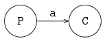
A screenshot showing a Chi model and simulation with visualization:
Chi Tutorial
This manual explains using the Chi modeling language.
Topics
-
Introduction (global description of the aims of the language)
-
Basics: Elementary knowledge needed for writing and understanding Chi programs. Start here to learn the language!
-
Data types (explanation of all kinds of data and their operations)
-
Statements (available process statements)
-
Functions (how to use functions)
-
Input and output (reading/writing files, displaying output)
-
-
Programming: How to specify parallel executing processes using the Chi language.
-
Modeling stochastic behavior (how to model varying behavior)
-
Processes (creating and running processes)
-
Channels (connecting processes with each other)
-
-
Modeling: Modeling a real system with Chi.
-
Buffers (modeling temporary storage of items)
-
Servers (modeling machines)
-
Conveyors (modeling conveyor belts)
-
Experiments (performing simulation experiments)
-
-
Visualization: Making an animated graphical display of a system with the Chi simulator.
-
SVG visualization (how to attach an SVG visualization)
-
SVG example (an SVG example)
-
Introduction
The topic is modeling of the operation of (manufacturing) systems, e.g. semiconductor factories, assembly and packaging lines, car manufacturing plants, steel foundries, metal processing shops, beer breweries, health care systems, warehouses, order-picking systems. For a proper functioning of these systems, these systems are controlled by operators and electronic devices, e.g. computers.
During the design process, engineers make use of (analytical) mathematical models, e.g. algebra and probability theory, to get answers about the operation of the system. For complex systems, (numerical) mathematical models are used, and computers perform simulation experiments, to analyze the operation of the system. Simulation studies give answers to questions like:
-
What is the throughput of the system?
-
What is the effect of set-up time in a machine?
-
How will the batch size of an order influence the flow time of the product-items?
-
What is the effect of more surgeons in a hospital?
The operation of a system can be described, e.g. in terms of or operating processes.
An example of a system with parallel operating processes is a manufacturing line, with a number of manufacturing machines, where product-items go from machine to machine. A surgery room in a hospital is a system where patients are treated by teams using medical equipment and sterile materials. A biological system can be described by a number of parallel processes, where, e.g. processes transform sugars into water and carbon-dioxide producing energy. In all these examples, processes operate in parallel to complete a task, and to achieve a goal. Concurrency is the dominant aspect in these type of systems, and as a consequence this holds too for their models.
The operating behavior of parallel processes can be described by different formalisms, e.g. automata, Petri-nets or parallel processes. This text uses the programming language Chi, which is an instance of a parallel processes formalism.
A system is abstracted into a model, with cooperating processes, where processes are connected to each other via channels. The channels are used for exchanging material and information. Models of the above mentioned examples consist of a number of concurrent processes connected by channels, denoting the flow of products, patients or personnel.
In Chi, communication takes place in a synchronous manner. This means that communication between a sending process, and a receiving process takes place only when both processes are able to communicate. Processes and channels can dynamically be altered. To model times, like inter-arrival times and server processing times, the language has a notation of time.
The rationale behind the language is that models for the analysis of a system should be
-
formal (exactly one interpretation, every reader attaches the same meaning to the model),
-
easily writable (write the essence of the system in a compact way),
-
easily readable (non-experts should be able to understand the model),
-
and easily extensible (adding more details in one part should not affect other parts).
Verification of the models to investigate the properties of the model should be relatively effortless. (A model has to preserve some properties of the real system otherwise results from the simulation study have no relation with the system being modeled. The language must allow this verification to take place in a simple manner.)
Experiments should be performed in an straightforward manner. (Minimizing the effort in doing simulation studies, in particular for large systems, makes the language useful.)
Finally, the used models should be usable for the supervisory (logic) control of the systems (simulation studies often provide answers on how to control a system in a better way, these answers should also work for the modeled system).
Chi in a nutshell
During the past decades, the ancestors of Chi have been used with success, for the analysis of a variety of (industrial) systems. Based on this experience, the language Chi has been completely redesigned, keeping the strong points of the previous versions, while making it more powerful for advanced users, and easier to access for non-experts.
Its features are:
-
A system (and its control) is modeled as a collection of parallel running processes, communicating with each other using channels.
-
Processes do not share data with other processes and channels are synchronous (sending and receiving is always done together at the same time), making reasoning about process behavior easier.
-
Processes and channels are dynamic, new processes can be created as needed, and communication channels can be created or rerouted.
-
Variables can have elementary values such as boolean, integer or real numbers, to high level structured collections of data like lists, sets and dictionaries to model the data of the system. If desired, processes and channels can also be part of that data.
-
A small generic set of statements to describe algorithms, assignment, if, while, and for statements. This set is relatively easy to explain to non-experts, allowing them to understand the model, and participate in the discussions.
-
Tutorials and manuals demonstrate use of the language for effective modeling of system processes. More detailed modeling of the processes, or custom tailoring them to the real situation, has no inherent limits.
-
Time and (quasi-) random number generation distributions are available for modeling behavior of the system in time.
-
Likewise, measurements to derive performance indicators of the modeled system are integrated in the model. Tutorials and manuals show basic use. The integration allows for custom solutions to obtain the needed data in the wanted form.
-
Input and output facilities from and to the file system exists to support large simulation experiments.
Exercises
-
Install the Chi programming environment at your computer.
-
Test your first program.
-
Construct the following program in a project in your workspace:
model M(): writeln("It works!") end -
Compile, and simulate the model as explained in the tool manual (in Compile and simulate).
-
Try to explain the result.
-
-
Test a program with model parameters.
-
Construct the following program in the same manner:
model M(string s): write("%s\n") end -
Simulate the model, where you have to set the Model instance text to
M("OOPS")in the dialog box of the simulator. -
Try to explain the result.
-
Data types
The language is a statically typed language, which means that all variables and values in a model have a single fixed type.
All variables must be declared in the program.
The declaration of a variable consists of the type, and the name, of the variable.
The following fragment shows the declaration of two elementary data types, integer variable i and real variable r:
...
int i;
real r;
...
The ellipsis (...) denotes that non-relevant information is left out from the fragment.
The syntax for the declaration of variables is similar to the language C.
All declared variables are initialized, variables i and r are both initialized to zero.
An expression, consisting of operators, e.g. plus (+), times (*), and operands, e.g. i and r, is used to calculate a new value.
The new value can be assigned to a variable by using an assignment statement.
An example with four variables, two expressions and assignment statements is:
...
int  i = 2, j;
real r = 1.50, s;

j = 2 * i + 1;
s = r / 2;
...
The value of variable j becomes 5, and the value of s becomes 0.75.
Statements are described in Statements.
Data types are categorized in five different groups: elementary types, tuple types, container types, custom types, and distribution types. Elementary types are types such as Boolean, integer, real or string. Tuple types contain at least one element, where each element can be of different type. In other languages tuple types are called records (Pascal) or structures (C). Variables with a container type (a list, set, or dictionary) contain many elements, where each element is of the same type. Custom types are created by the user to enhance the readability of the model. Distributions types are types used for the generation of distributions from (pseudo-) random numbers. They are covered in Modeling stochastic behavior.
Elementary types
The elementary data types are Booleans, numbers and strings. The language provides the elementary data types:
-
boolfor booleans, with valuesfalseandtrue. -
enumfor enumeration types, for exampleenum FlagColors = {red, white, blue}, -
intfor integers, e.g.-7,20,0. -
realfor reals, e.g.3.14,7.0e9. -
stringfor text strings, e.g."Hello","world".
Booleans
A boolean value has two possible values, the truth values.
These truth values are false and true.
The value false means that a property is not fulfilled.
A value true means the presence of a property.
Boolean variables are initialized with the value false.
In mathematics, various symbols are used for unary and binary boolean operators.
These operators are also present in Chi.
The most commonly used boolean operators are not, and, and or.
The names of the operators, the symbols in mathematics and the symbols in the language are presented in the following table:
| Operator | Math | Chi |
|---|---|---|
boolean not |
¬ |
|
boolean and |
∧ |
|
boolean or |
∨ |
|
Examples of boolean expressions are the following.
If z equals true, then the value of (not z) equals false.
If s equals false, and t equals true, then the value of the expression (s or t) becomes true.
The result of the unary not, the binary and and or operators, for two variables p and q is given in the following table:
p |
q |
not p |
p and q |
p or q |
|---|---|---|---|---|
|
|
|
|
|
|
|
|
|
|
|
|
|
|
|
|
|
|
|
If p = true and q = false, we find for p or q the value true (third line in the table).
Enumerations
Often there are several variants of entities, like types of products, available resources, available machine types, and so on.
One way of coding them is give each a unique number, which results in code with a lot of small numbers that are not actually numbers, but refer to one variant.
Another way is to give each variant a name (which often already exists), and use those names instead.
For example, to model a traffic light:
enum TrafficColor = {RED, ORANGE, GREEN};

TrafficColor light = RED;
The enum TrafficColor line lists the available traffic colors.
With this definition, a new type TrafficColor is created, which you can use like any other type.
The line TrafficColor light = RED; creates a new variable called light and initializes it to the value RED.
Numbers
In the language, two types of numbers are available: integer numbers and real numbers.
Integer numbers are whole numbers, denoted by type int e.g. 3, -10, 0.
Real numbers are used to present numbers with a fraction, denoted by type real.
E.g. 3.14, 2.7e6 (the scientific notation for 2.7 million).
Note that real numbers must either have a fraction or use the scientific notation, to let the computer know you mean a real number (instead of an integer number).
Integer variables are initialized with 0.
Real variables are initialized with 0.0.
For numbers, the normal arithmetic operators are defined. Expressions can be constructed with these operators. The arithmetic operators for numbers are listed in the following table:
| Operator name | Notation | Comment |
|---|---|---|
unary plus |
|
|
unary minus |
|
|
raising to the power |
|
Always a |
multiplication |
|
|
real division |
|
Always a |
division |
|
For |
modulo |
|
For |
addition |
|
|
subtraction |
|
The priority of the operators is given from high to low.
The unary operators have the strongest binding, and the + and - the weakest binding.
So, -3^2 is read as (-3)^2 and not -(3^2), because the priority rules say that the unary operator binds stronger than the raising to the power operator.
Binding in expressions can be changed by the use of parentheses.
The integer division, denoted by div, gives the biggest integral number smaller or equal to x / y.
The integer remainder, denoted by mod, gives the remainder after division x - y * (x div y).
So, 7 div 3 gives 2 and -7 div 3 gives -3, 7 mod 3 gives 1 and -7 mod 3 gives 2.
The rule for the result of an operation is as follows.
The real division and raising to the power operations always produce a value of type real.
Otherwise, if both operands (thus x and y) are of type int, the result of the operation is of type int.
If one of the operands is of type real, the result of the operation is of type real.
Conversion functions exist to convert a real into an integer.
The function ceil converts a real to the smallest integer value not less than the real, the function floor gives the biggest integer value smaller than or equal to the real, and the function round rounds the real to the nearest integer value (or up, if it ends on .5).
Between two numbers a relational operation can be defined.
If for example variable x is smaller than variable y, the expression x < y equals true.
The relational operators, with well-known semantics, are listed in the following table:
| Name | Operator |
|---|---|
less than |
|
at most |
|
equals |
|
differs from |
|
at least |
|
greater than |
|
Strings
Variables of type string contains a sequence of characters.
A string is enclosed by double quotes.
An example is "Manufacturing line".
Strings can be composed from different strings.
The concatenation operator (+) adds one string to another, for example "One" + " " + "string" gives "One string".
Moreover the relational operators (<, <=, ==, != >=, and >) can be used to compare strings alphabetically, e.g. "a" < "aa" < "ab" < "b".
String variables are initialized with the empty string "".
Tuple types
Tuple types are used for keeping several (related) kinds of data together in one variable, e.g. the name and the age of a person.
A tuple variable consists of a number of fields inside the tuple, where the types of these fields may be different.
The number of fields is fixed.
One operator, the projection operator denoted by a dot (.), is defined for tuples.
It selects a field in the tuple for reading or assigning.
Notation
A type person is a tuple with two fields, a 'name' field of type string, and an 'age' field of type int, is denoted by:
type person = tuple(string name; int age)Operator
A projection operator fetches a field from a tuple. We define two persons:
person eva  = ("eva" , 29),
       adam = ("adam", 27);
And we can speak of eva.name and adam.age, denoting the name of eva ("eva") and the age of adam (27).
We can assign a field in a tuple to another variable:
ae = eva.age;
eva.age = eva.age + 1;
This means that the age of eva is assigned tot variable ae, and the new age of eva becomes eva.age + 1.
By using a multi assignment statement all values of a tuple can be copied into separate variables:
string name;
int age;

name, age = eva
This assignment copies the name of eva into variable name of type string and her age into age of type int.
Container types
Lists, sets and dictionaries are container types. A variable of this type contains zero or more identical elements. Elements can be added or removed in variables of these types. Variables of a container type are initialized with zero elements.
Sets are unordered collections of elements. Each element value either exists in a set, or it does not exist in a set. Each element value is unique, duplicate elements are silently discarded. A list is an ordered collection of elements, that is, there is a first and a last element (in a non-empty list). A list also allows duplicate element values. Dictionaries are unordered and have no duplicate value, just like sets, but you can associate a value (of a different type) with each element value.
Lists are denoted by a pair of (square) brackets.
For example, [7, 8, 3] is a list with three integer elements.
Since a list is ordered, [8, 7, 3] is a different list.
With empty lists, the computer has to know the type of the elements, e.g. <int>[] is an empty list with integer elements.
The prefix <int> is required in this case.
Sets are denoted by a pair of (curly) braces, e.g. {7, 8, 3} is a set with three integer elements.
As with lists, for an empty set a prefix is required, for example <string>{} is an empty set with strings.
A set is an unordered collection of elements.
The set {7, 8, 3} is a set with three integer numbers.
Since order of the elements does not matter, the same set can also be written as {8, 3, 7} (or in one of the four other orders).
In addition, each element in a set is unique, the set {8, 7, 8, 3} is equal to the set {7, 8, 3}.
For readability, elements in a set are normally written in increasing order, for example {3, 7, 8}.
Dictionaries are denoted by a pair of (curly) braces, whereby an element value consists of two parts, a 'key' and a 'value' part.
The two parts separated by a colon (:).
For example {"jim" : 32, "john" : 34} is a dictionary with two elements.
The first element has "jim" as key part and 32 as value part, the second element has "john" as key part and 34 as value part.
The key parts of the elements work like a set, they are unordered and duplicates are silently discarded.
A value part is associated with its key part.
In this example, the key part is the name of a person, while the value part keeps the age of that person.
Empty dictionaries are written with a type prefix just like lists and sets, e.g. <string:int>{}.
Container types have some built-in functions in common (Functions are described in Functions):
-
The function
sizegives the number of elements in a variable, for examplesize([7, 8, 3])yields 3;size({7, 8})results in 2;size({"jim":32})gives 1 (an element consists of two parts).
-
The function
emptyyieldstrueif there are no elements in variable. E.g.empty(<string>{})with an empty set of typestringis true. (Here the typestringis needed to determine the type of the elements of the empty set.)
-
The function
popextracts a value from the provided collection and returns a tuple with that value, and the collection minus the value.For lists, the first element of the list becomes the first field of the tuple. The second field of the tuple becomes the list minus the first list element. For example:
pop([7, 8, 3]) -> (7, [8, 3])The
->above denotes 'yields'. The value of the list is split into a 'head' (the first element) and a 'tail' (the remaining elements).For sets, the first field of the tuple becomes the value of an arbitrary element from the set. The second field of the tuple becomes the original set minus the arbitrary element. For example, a
popon the set{8, 7, 3}has three possible answers:pop({8, 7, 3}) -> (7, {3, 8}) or pop({8, 7, 3}) -> (3, {7, 8}) or pop({8, 7, 3}) -> (8, {3, 7})Performing a
popon a dictionary follows the same pattern as above, except 'a value from the collection' are actually a key item and a value item. In this case, thepopfunction gives a three-tuple as result. The first field of the tuple becomes the key of the extracted element, the second field of the tuple becomes the value of the element, and the third field of the tuple contains the dictionary except for the extracted element. Examples:pop({"a" : 32, "b" : 34}) -> ("a", 32, {"b" : 34}) or pop({"a" : 32, "b" : 34}) -> ("b", 34, {"a" : 32})
Lists
A list is an ordered collection of elements of the same type. They are useful to model anything where duplicate values may occur or where order of the values is significant. Examples are waiting customers in a shop, process steps in a recipe, or products stored in a warehouse. Various operations are defined for lists.
An element can be fetched by indexing.
This indexing operation does not change the content of the variable.
The first element of a list has index 0.
The last element of a list has index size(xs) - 1.
A negative index, say m, starts from the back of the list, or equivalently, at offset size(xs) + m from the front.
You cannot index non-existing elements.
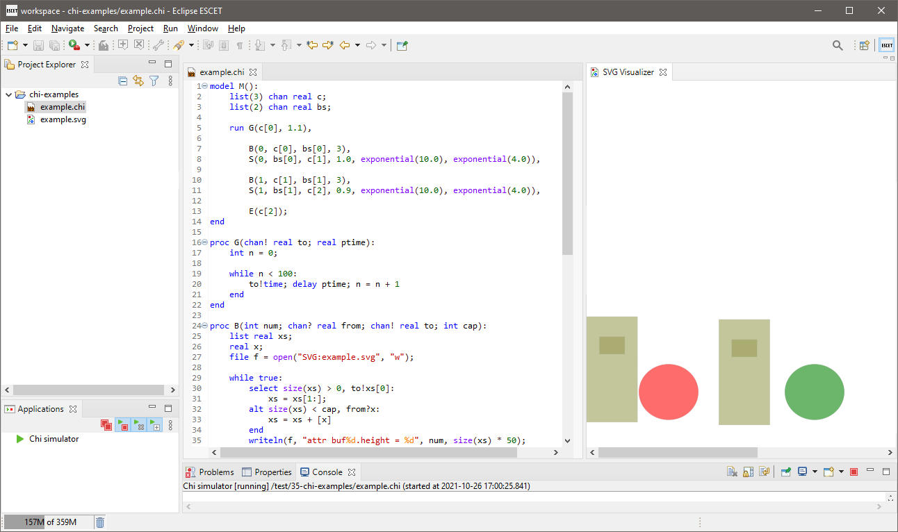
Some examples, with xs = [7, 8, 3, 5, 9] are:
xs[0]  -> 7
xs[3]  -> 5
xs[5]  -> ERROR (there is no element at position 5)
xs[-1] -> xs[5 - 1] -> xs[4] -> 9
xs[-2] -> xs[5 - 2] -> xs[3] -> 5
In the figure below, the list with indices is visualized.
A common name for the first element of a list (i.e., x[0]) is the head of a list.
Similarly, the last element of a list (xs[-1]) is also known as head right.
A part of a list can be fetched by slicing. The slicing operation does not change the content of the list, it copies a contiguous sequence of a list. The result of a slice operation is again a list, even if the slice contains just one element.
Slicing is denoted by xs[i:j].
The slice of xs[i:j] is defined as the sequence of elements with index k such that i <= k < j.
Note the upper bound j is noninclusive.
If i is omitted use 0.
If j is omitted use size(xs).
If i is greater than or equal to j, the slice is empty.
If i or j is negative, the index is relative to the end of the list: size(xs) + i or size(xs) + j is substituted.
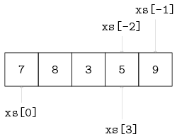
Some examples with xs = [7, 8, 3, 5, 9]:
xs[1:3] -> [8, 3]
xs[:2]  -> [7, 8]
xs[1:]  -> [8, 3, 5, 9]
xs[:-1] -> [7, 8, 3, 5]
xs[:-3] -> [7, 8]
The list of all but the first elements (xs[1:]) is often called tail and xs[:-1] is also known as tail right.
Below, the slicing operator is visualized:
Two lists can be 'glued' together into a new list.
The glue-ing or concatenation of a list with elements 7, 8, 3 and a list with elements 5, and 9 is denoted by:
[7, 8, 3] + [5, 9] -> [7, 8, 3, 5, 9]An element can be added to a list at the rear or at the front.
The action is performed by transforming the element into a list and then concatenate these two lists.
In the next example the value 5 is added to the rear, respectively the front, of a list:
[7, 8, 3] + [5] -> [7, 8, 3, 5]
[5] + [7, 8, 3] -> [5, 7, 8, 3]
Elements also can be removed from a list.
The del function removes by position, e.g. del(xs, 2) returns the list xs without its third element (since positions start at index 0).
Removing a value by value can be performed by the subtraction operator -.
For instance, consider the following subtractions:
[1, 4, 2, 4, 5] - [2] -> [1, 4, 4, 5]
[1, 4, 2, 4, 5] - [4] -> [1, 2, 4, 5]
[1, 4, 2, 4, 5] - [8] -> [1, 4, 2, 4, 5]
Every element in the list at the right is searched in the list at the left, and if found, the first occurrence is removed.
In the first example, element 2 is removed.
In the second example, only the first value 4 is removed and the second value (at position 3) is kept.
In the third example, nothing is removed, since value 8 is not in the list at the left.
When the list at the right is longer than one element, the operation is repeated.
For example, consider xs - ys, whereby xs = [1, 2, 3, 4, 5] and ys = [6, 4, 2, 3].
The result is computed as follows:
    [1, 2, 3, 4, 5] - [6, 4, 2, 3]
-> ([1, 2, 3, 4, 5] - [6]) - [4, 2, 3]
->  [1, 2, 3, 4, 5] - [4, 2, 3]
-> ([1, 2, 3, 4, 5] - [4]) - [2, 3]
->  [1, 2, 3,    5] - [2, 3]
-> ([1, 2, 3,    5] - [2]) - [3]
->  [1,    3,    5] - [3]
-> [1,5]
Lists have two relational operators, the equal operator and the not-equal operator.
The equal operator (==) compares two lists.
If the lists have the same number of elements and all the elements are pair-wise the same, the result of the operation is true, otherwise false.
The not-equal operator (!=) does the same check, but with an opposite result.
Some examples, with xs = [7, 8, 3]:
xs == [7, 8, 3] -> true
xs == [7, 7, 7] -> false
The membership operator (in) checks if an element is in a list.
Some examples, with xs = [7, 8, 3]:
6 in xs -> false
7 in xs -> true
8 in xs -> true
Initialization
A list variable is initialized with a list with zero elements, for example in:
list int xs;The initial value of xs equals <int>[].
A list can be initialized with a number, denoting the number of elements in the list:
list(2) int ysThis declaration creates a list with 2 elements, whereby each element of type int is initialized.
The initial value of ys equals [0, 0].
Another example with a list of lists:
list(4) list(2) int zmThis declaration initializes variable zm with the value [ [0, 0], [0, 0], [0, 0], [0, 0] ].
Sets
Set operators for union, intersection and difference are present. The table below gives the name, the mathematical notation and the notation in the Chi language:
| Operator | Math | Chi |
|---|---|---|
set union |
∪ |
|
set intersection |
∩ |
|
set difference |
∖ |
|
The union of two sets merges the values of both sets into one, that is, the result is the collection of values that appear in at least one of the arguments of the union operation. Some examples:
{3, 7, 8} + {5, 9} -> {3, 5, 7, 8, 9}All permutations with the elements 3, 5, 7, 8 and 9 are correct (sets have no order, all permutations are equivalent).
To keep sets readable the elements are sorted in increasing order in this tutorial.
Values that occur in both arguments, appear only one time in the result (sets silently discard duplicate elements). For example:
{3, 7, 8} + {7, 9} -> {3, 7, 8, 9}The intersection of two sets gives a set with the common elements, that is, all values that occur in both arguments. Some examples:
{3, 7, 8} * {5, 9} -> <int>{}   # no common element
{3, 7, 8} * {7, 9} -> {7}       # only 7 in common
Set difference works much like subtraction on lists, except elements occur at most one time (and have no order). The operation computes 'remaining elements'. The result is a new set containing all values from the first set which are not in the second set. Some examples:
{3, 7, 8} - {5, 9} -> {3, 7, 8}
{3, 7, 8} - {7, 9} -> {3, 9}
The membership operator in works on sets too:
3 in {3, 7, 8} -> true
9 in {3, 7, 8} -> false
Dictionaries
Elements of dictionaries are stored according to a key, while lists elements are ordered by a (relative) position, and set elements are not ordered at all. A dictionary can grow and shrink by adding or removing elements respectively, like a list or a set. An element of a dictionary is accessed by the key of the element.
The dictionary variable d of type dict(string : int) is given by:
dict (string : int) d =
    {"jim"  : 32,
     "john" : 34,
     "adam" : 25}
Retrieving values of the dictionary by using the key:
d["john"] -> 34
d["adam"] -> 25
Using a non-existing key to retrieve a value results in a error message.
A new value can be assigned to the variable by selecting the key of the element:
d["john"] = 35This assignment changes the value of the "john" item to 35.
The assignment can also be used to add new items:
d["lisa"] = 19Membership testing of keys in dictionaries can be done with the in operator:
"jim" in d -> true
"peter" in d -> false
Merging two dictionaries is done by adding them together. The value of the second dictionary is used when a key exists in both dictionaries:
{1 : 1, 2 : 2} + {1 : 5, 3 : 3} -> {1 : 5, 2 : 2, 3 : 3}The left dictionary is copied, and updated with each item of the right dictionary.
Removing elements can be done with subtraction, based on key values.
Lists and sets can also be used to denote which keys should be removed.
A few examples for p is {1 : 1, 2 : 2}:
p - {1 : 3, 5 : 5} -> {2 : 2}
p - {1, 7} -> {2 : 2}
p - [2, 8] -> {1 : 1}
Subtracting keys that do not exist in the left dictionary is allowed and has no effect.
Custom types
To structure data the language allows the creation of new types.
The definition can only be done at global level, that is, outside any proc, func, model, or xper definition.
Types can be used as alias for elementary data types to increase readability, for example a variable of type item:
type item = real;Variables of type item are, e.g.:
item box, product;

box = 4.0; product = 120.5;
This definition creates the possibility to speak about an item.
Types also can be used to make combinations of other data types, e.g. a recipe:
type step   = tuple(string name; real process_time),
     recipe = tuple(int id; list step steps);
A type step is defined by a tuple with two fields, a field with name of type string, denoting the name of the step, and a field with process_time of type real, denoting the duration of the (processing) step.
The step definition is used in the type recipe.
Type recipe is defined by a tuple with two fields, an id of type int, denoting the identification number, and a field steps of type list step, denoting a list of single steps.
Variables of type recipe are, e.g.:
recipe plate, bread;
plate = (34, [("s", 10.8), ("w", 13.7), ("s", 25.6)]);
bread = (90, [("flour", 16.3), ("yeast", 6.9)]);
Exercises
-
Exercises for integer numbers. What is the result of the following expressions:
-5 ^ 3 -5 * 3 5 mod 3 -
Exercises for tuples. Given are tuple type
boxand variablexof typebox:type box = tuple(string name; real weight); box x = ("White", 12.5);What is the result of the following expressions:
x.name x.real x -
Exercises for lists. Given is the list
xs = [0,1,2,3,4,5,6]. Determine the outcome of:xs[0] xs[1:] size(xs) xs + [3] [4,5] + xs xs - [2,2,3] xs - xs[2:] xs[0] + (xs[1:])[0]
Statements
There are several kinds of statements, such as assignment statements, choice statements (select and if statements), and loop statements (while and for statements).
Semicolons are required after statements, except at the end of a sequence (that is, just before an end keyword and after the last statement) or after the keyword end.
In this text semicolons are omitted before end.
The assignment statement
An assignment statement is used to assign values to variables. An example:
y = x + 10This assignment consists of a name of the variable (y), an assignment symbol (=), and an expression (x + 10) yielding a value.
For example, when x is 2, the value of the expression is 12.
Execution of this statement copies the value to the y variable, immediately after executing the assignment, the value of the y variable is 10 larger than the value of the x variable at this point of the program.
The value of the y variable will not change until the next assignment to y, for example, performing the assignment x = 7 has no effect on the value of the y variable.
An example with two assignment statements:
i = 2;
j = j + 1
The values of i becomes 2, and the value of j is incremented.
Independent assignments can also be combined in a multi-assignment, for example:
i, j = 2, j + 1The result is the same as the above described example, the first value goes into the first variable, the second value into the second variable, etc.
In an assignment statement, first all expression values are computed before any assignment is actually done.
In the following example the values of x and y are swapped:
x, y = y, x;
The if statement
The if statement is used to express decisions. An example:
if x < 0:
    y = -x
end
If the value of x is negative, assign its negated value to y.
Otherwise, do nothing (skip the y = -x assignment statement).
To perform a different statement when the decision fails, an if-statement with an else alternative can be used.
It has the following form.
An example:
if a > 0:
    c = a
else:
    c = b
end
If a is positive, variable c gets the value of a, otherwise it gets the value of b.
In some cases more alternatives must be tested.
One way of writing it is by nesting an if-statement in the else alternative of the previous if-statement, like:
if i < 0:
    writeln("i < 0")
else:
    if i == 0:
        writeln("i = 0")
    else:
        if i > 0 and i < 10:
            writeln("0 < i < 10")
        else:
            # i must be greater or equal 10
            writeln("i >= 10")
        end
    end
end
This tests i < 0.
If it fails, the else is chosen, which contains a second if-statement with the i == 0 test.
If that test also fails, the third condition i > 0 and i < 10 is tested, and one of the writeln statements is chosen.
The above can be written more compactly by combining an else-part and the if-statement that follows, into an elif part.
Each elif part consists of a boolean expression, and a statement list.
Using elif parts results in:
if i < 0:
    writeln("i < 0")
elif i == 0:
    writeln("i = 0")
elif i > 0 and i < 10:
    writeln("0 < i < 10")
else:
    # i must be greater or equal 10
    writeln("i >= 10")
end
Each alternative starts at the same column, instead of having increasing indentation. The execution of this combined statement is still the same, an alternative is only tested when the conditions of all previous alternatives fail.
Note that the line # i must be greater or equal 10 is a comment to clarify when the alternative is chosen.
It is not executed by the simulator.
You can write comments either at a line by itself like above, or behind program code.
It is often useful to clarify the meaning of variables, give a more detailed explanation of parameters, or add a line of text describing what the purpose of a block of code is from a birds-eye view.
The while statement
The while statement is used for repetitive execution of the same statements, a so-called loop.
A fragment that calculates the sum of 10 integers, 10, 9, 8, ..., 3, 2, 1, is:
int i = 10, sum;

while i > 0:
    sum = sum + i; i = i - 1
end
Each iteration of a while statement starts with evaluating its condition (i > 0 above).
When it holds, the statements inside the while (the sum = sum + i; i = i - 1 assignments) are executed (which adds i to the sum and decrements i).
At the end of the statements, the while is executed again by evaluating the condition again.
If it still holds, the next iteration of the loop starts by executing the assignment statements again, etc.
When the condition fails (i is equal to 0), the while statement ends, and execution continues with the statement following end.
A fragment with an infinite loop is:
while true:
    i = i + 1;
    ...
end
The condition in this fragments always holds, resulting in i getting incremented 'forever'.
Such loops are very useful to model things you switch on but never off, e.g. processes in a factory.
A fragment to calculate z = x ^ y, where z and x are of type real, and y is of type integer with a non-negative value, showing the use of two while loops, is:
real x; int y; real z = 1;

while y > 0:
    while y mod 2 == 0:
        y = y div 2; x = x * x
    end;
    y = y - 1; z = x * z
end
A fragment to calculate the greatest common divisor (GCD) of two integer numbers j and k, showing the use of if and while statements, is:
while j != k:
    if j > k:
        j = j - k
    else:
        k = k - j
    end
end
The symbol != stands for 'differs from' ('not equal').
The for statement
The while statement is useful for looping until a condition fails.
The for statement is used for iterating over a collection of values.
A fragment with the calculation of the sum of 10 integers:
int sum;

for i in range(1, 11):
    sum = sum + i
end
The result of the expression range(1, 11) is a list whose items are consecutive integers from 1 (included) up to 11 (excluded): [1, 2, 3, ..., 9, 10].
The following example illustrates the use of the for statement in relation with container-type variables. Another way of calculating the sum of a list of integer numbers:
list int xs = [1, 2, 3, 5, 7, 11, 13];
int sum;

for x in xs:
    sum = sum + x
end
This statement iterates over the elements of list xs.
This is particularly useful when the value of xs may change before the for statement.
Notes
In this chapter the most used statements are described. Below are a few other statements that may be useful some times:
-
Inside loop statements, the break and continue statements are allowed. The
breakstatements allows 'breaking out of a loop', that is, abort a while or a for statement. Thecontinuestatement aborts execution of the statements in a loop. It 'jumps' to the start of the next iteration.
-
A rarely used statement is the
passstatement. It’s like anx = xassignment statement, but more clearly expresses 'nothing is done here'.
Exercises
-
Study the Chi specification below and explain why, though it works, it is not an elegant way of modeling the selection. Make a suggestion for a shorter, more elegant version of:
model M(): int i = 3; if (i < 0) == true: write("%d is a negative number\n", i); elif (i <= 0) == false: write("%d is a positive number\n", i); end end -
Construct a list with the squares of the integers 1 to 10.
-
using a
forstatement, and -
using a
whilestatement.
-
-
Write a program that
-
Makes a list with the first 50 prime numbers.
-
Extend the program with computing the sum of the first 7 prime numbers.
-
Extend the program with computing the sum of the last 11 prime numbers.
-
Functions
In a model, computations must be performed to process the information that is sent around.
Short and simple calculations are written as assignments between the other statements, but for longer computations or computations that are needed at several places in the model, a more encapsulated environment is useful, a function.
In addition, the language comes with a number of built-in functions, such as size or empty on container types.
An example:
func real mean(list int xs):
    int sum;

    for x in xs:
        sum = sum + x
    end;
    return sum / size(xs)
end
The func keyword indicates it is a function.
The name of the function is just before the opening parenthesis, in this example mean.
Between the parentheses, the input values (the formal parameters) are listed.
In this example, there is one input value, namely list int which is a list of integers.
Parameter name xs is used to refer to the input value in the body of the function.
Between func and the name of the function is the type of the computation result, in this case, a real value.
In other words, this mean function takes a list of integers as input, and produces a real value as result.
The colon at the end of the first line indicates the start of the computation.
Below it are new variable declarations (int sum), and statements to compute the value, the function algorithm.
The return statement denotes the end of the function algorithm.
The value of the expression behind it is the result of the calculation.
This example computes and returns the mean value of the integers of the list.
Use of a function (application of a function) is done by using its name, followed by the values to be used as input (the actual parameters). The above function can be used like:
m = mean([1, 3, 5, 7, 9])The actual parameter of this function application is [1, 3, 5, 7, 9].
The function result is (1 + 3 + 5 + 7 + 9)/5 (which is 5.0), and variable m becomes 5.0.
A function is a mathematical function: the result of a function is the same for the same values of input parameters.
A function has no side-effect, and it cannot access variables outside the body.
For example, it cannot access time (explained in Servers with time) directly, it has to be passed in through the parameter list.
A function that calculates the sign of a real number, is:
func int sign(real r):
    if r < 0:
        return -1
    elif r = 0:
        return  0
    end;
    return  1
end
The sign function returns:
-
if
ris smaller than zero, the value minus one; -
if
requals zero, the value zero; and -
if
ris greater than zero, the value one.
The computation in a function ends when it encounters a return statement.
The return 1 at the end is therefore only executed when both if conditions are false.
Sorted lists
The language allows recursive functions as well as higher-order functions. Explaining them in detail is beyond the scope of this tutorial, but these functions are useful for making and maintaining sorted lists. Such a sorted list is useful for easily getting the smallest (or largest) item from a collection, for example the order with the nearest deadline.
To sort a list, the first notion that has to be defined is the desired order, by making a function of the following form:
func bool decreasing(int x, y):
    return x >= y
end
The function is called predicate function.
It takes two values from the list (two integers in this case), and produces a boolean value, indicating whether the parameters are in the right order.
In this case, the function returns true when the first parameter is larger or equal than the second parameter, that is, larger values must be before smaller values (for equal values, the order does not matter).
This results in a list with decreasing values.
The requirements on any predicate function f are:
-
If
x != y, eitherf(x, y)must hold orf(y, x)must hold, but not both. (Unequal values must have a unique order.) -
If
x == y, bothf(x, y)andf(y, x)must hold. (Equal values can be placed in arbitrary order.) -
For values
x,y, andz, iff(x, y)holds andf(y, z)holds (that isx >= yandy >= z), thenf(x, z)must also hold (that is,x >= zshould also be true).
(The order between x and z must be stable, even when you compare with an intermediate value y between x and z.)
These requirements hold for functions that test on <= or >= between two values, like above.
If you do not provide a proper predicate function, the result may not be sorted as you expect, or the simulator may abort when it fails to find a proper sorting order.
Sort
The first use of such a predicate function is for sorting a list.
For example list [3, 8, 7] is sorted decreasingly (larger numbers before smaller numbers) with the following statement:
ys = sort([3, 8, 7], decreasing)Sorting is done with the sort function, it takes two parameters, the list to sort, and the predicate function.
(There are no parentheses () behind decreasing!) The value of list ys becomes [8, 7, 3].
Another sorting example is a list of type tuple(int number, real slack), where field number denotes the number of an item, and field slack denotes the slack time of the item.
The list should be sorted in ascending order of the slack time.
The type of the item is:
type item = tuple(int number, real slack);The predicate function spred is defined by:
func bool spred(item x, y):
    return x.slack <= y.slack
end
Function spred returns true if the two elements are in increasing order in the list, otherwise false.
Note, the parameters of the function are of type item.
Given a variable ps equal to [(7, 21.6), (5, 10.3), (3, 35.8)].
The statement denoting the sorting is:
qs = sort(ps, spred)variable qs becomes [(5, 10.3), (7, 21.6), (3, 35.8)].
Insert
Adding a new value to a sorted list is the second use of higher-order functions.
The simplest approach would be to add the new value to the head or rear of the list, and sort the list again, but sorting an almost sorted list is very expensive.
It is much faster to find the right position in the already sorted list, and insert the new value at that point.
This function also exists, and is named insert.
An example is (assume xs initially contains [3,8]):
xs = insert(xs, 7, increasing)where increasing is:
func bool increasing(int x, y):
    return x <= y
end
The insert call assigns the result [3,7,8] as new value to xs, 7 is inserted in the list.
Input and output
A model communicates with the outside world, e.g. screen and files, by the use of read statements for input of data, and write statements for output of data.
The read function
Data can be read from the command line or from a file by read functions. A read function requires a type value for each parameter to be read. An example:
int i; string s;

i = read(int);
s = read(string);
Two values, an integer value and a string value are read from the command line. On the command line the two values are typed:
1 "This is a string"Variable i becomes 1, and string s becomes "This is a string".
The double quotes are required!
Parameter values are separated by a space or a tabular stop.
Putting each value on a separate line also works.
Reading from a file
Data also can be read from files. An example fragment:
type row = tuple(string name; list int numbers);

file f;
int i;
list row rows;

f = open("data_file.txt", "r");
i = read(f, int);
rows = read(f, list row);
close(f)
Before a file can be used, the file has to be declared, and the file has to be opened by statement open.
Statement open has two parameters, the first parameter denotes the file name (as a string), and the second parameter describes the way the file is used.
In this case, the file is opened in a read-only mode, denoted by string "r".
Reading values works in the same way as before, except you cannot add new text in the file while reading it.
Instead, the file is processed sequentially from begin to end, with values separated from each other by white space (spaces, tabs, and new-lines).
You can read values of different types from the same file, as long as the value in the file matches with the type that you ask.
For example, the above Chi program could read the following data from data_file.txt:
21
[("abc", [7,21]),
 ("def", [8,31,47])]
After enough values have been read, the file should be closed with the statement close, with one parameter, the variable of the file.
If a file is still open after an experiment, the file is closed automatically before the program quits.
Advanced reading from a file
When reading from a file, the eof and eol functions can be used to obtain information about the white space around the values.
-
The
eof(end of file) function returnstrueif you have read the last value (that is, there are no more values to read). -
The
eol(end of line) function returnstrueif there are no more values at the current line. In particular, theeolfunction returnstruewhen the end of the file has been reached.
These functions can be used to customize reading of more complicated values.
As an example, you may want to read the same list row value as above, but without having all the comma’s, quotes, parentheses, and brackets of the literal value [("abc", [7,21]), ("def", [8,31,47])].
Instead, imagine having a file clean_data.txt with the following layout:
abc 7 21
def 8 31 47
Each line is one row.
It starts with a one-word string, followed by a list of integer numbers.
By using the eof and eol functions, you can read this file in the following way:
file f;
list row rows;
string name;
list int xs;

f = open("clean_data.txt", "r");
while not eof(f):
    name = read(f, string);
    xs = <int>[];
    while not eol(f): # Next value is at the same line.
        xs = xs + [read(f, int)];
    end
    rows = rows + [(name, xs)];
end
close(f);
Each line is processed individually, where eol is used to find out whether the last value of a line has been read.
The reading loop terminates when eof returns true.
Note that eol returns whether the current line has no more values.
It does not tell you how many lines down the next value is.
For example, an empty line inserted between the abc 7 21 line and the def 8 31 47 line is skipped silently.
If you want that information, you can use the newlines function instead.
The write statement
The write statement is used for output of data to the screen of the computer. Data can also be written to a file.
The first argument of write (or the second argument if you write to a file, see below) Is called the format string.
It is a template of the text to write, with 'holes' at the point where a data value is to be written.
Behind the format string, the data values to write are listed.
The first value is written in the first 'hole', the second value in the second 'hole' and so on.
The holes are also called place holders.
A place holder starts with % optionally followed by numbers or some punctuation (its meaning is explained below).
A place holder ends with a format specifier, a single letter like s or f.
An example:
int i = 5;

write("i equals %s", i)
In this example the text i equals 5 is written to the screen by the write statement.
The "i equals %s" format string defines what output is written.
All 'normal' characters are copied as-is.
The %s place holder is not copied.
Instead the first data value (in this case i) is inserted.
The s in the place holder is the format specifier.
It means 'print as string'.
The %s is a general purpose format specifier, it works with almost every type of data.
For example:
list dict(int:real) xs = [{1 : 5.3}];

write("%s", xs)
will output the contents of xs ({1 : 5.3}).
In general, this works nicely, but for numeric values a little more control over the output is often useful.
To this end, there are also format specifiers d for integer numbers, and f for real numbers.
An example:
int i = 5;
real r = 3.14;

write("Result:\n");
write("%4d/%8.2f", i, r);
This fragment has the effect that the values of i and r are written to the screen as follows:
Result:
   5/    3.14
The value of i is written in d format (as int value), and the value of r is written in f format (as real value).
The symbols d and f originate respectively from 'decimal', and 'floating point' numbers.
The numbers 4 respectively 8.2 denote that the integer value is written four positions wide (that is, 3 spaces and a 5 character), and that the real value is written eight positions wide, with two characters after the decimal point (that is, 4 spaces and the text 3.14).
A list of format specifiers is given in the following table:
| Format specifier | Description |
|---|---|
|
boolean value (outputs |
|
integer |
|
integer, at least ten characters wide |
|
real |
|
real, at least ten characters wide |
|
real, four characters after the decimal point |
|
real, at least ten characters wide with four characters after the decimal point |
|
character string |
|
the character |
Finally, there are also a few special character sequences called escape sequence which allow to write characters like horizontal tab (which means 'jump to next tab position in the output'), or newline (which means 'go to the next line in the output') in a string.
An escape sequence consists of two characters.
First a backslash character \, followed by a second character.
The escape sequences are presented in the following table:
| Sequence | Meaning |
|---|---|
|
new line |
|
horizontal tab |
|
the character |
|
the character |
An example is:
int i = 5, j = 10;
real r = 3.14;

write("Result:\n");
write("%6d\t%d\n\t%.2f\n", i, j, r);
The result looks like:
Result:
     5  10
        3.14
The value of j is written at the tab position, the output goes to the next line again at the first tab position, and outputs the value of r.
Writing to a file
Data can be written to a file, analog to the read function. A file has to be defined first, and opened for writing before the file can be used. An example:
file f;
int i;

f = open("output_file", "w");
write(f, "%s", i); write(f, "%8.2f", r);
close(f)
A file, in this case "output_file" is used in write-only mode, denoted by the character "w".
Opening a file for writing destroys its old contents (if the file already exists).
In the write statement, the first parameter must be the file, and the second parameter must be the format string.
After all data has been written, the file is closed by statement close.
If the file is still open after execution of the program, the file is closed automatically.
Modeling stochastic behavior
Many processes in the world vary a little bit each time they are performed. Setup of machines goes a bit faster or slower, patients taking their medicine takes longer this morning, more products are delivered today, or the quality of the manufactured product degrades due to a tired operator. Modeling such variations is often done with stochastic distributions. A distribution has a mean value and a known shape of variation. By matching the means and the variation shape with data from the system being modeled, an accurate model of the system can be obtained. The language has many stochastic distributions available, this chapter explains how to use them to model a system, and lists a few commonly used distributions. The full list is available in the reference manual at Distributions.
The following fragment illustrates the use of the random distribution to model a dice.
Each value of the six-sided dice is equally likely to appear.
Every value having the same probability of appearing is a property of the integer uniform distribution, in this case using interval [1, 7) (inclusive on the left side, exclusive on the right side).
The model is:
dist int dice = uniform(1,7);
int x, y;

x = sample dice;
y = sample dice;
writeln("x=%d, y=%d", x, y);
The variable dice is an integer distribution, meaning that values drawn from the distribution are integer numbers.
It is assigned an uniform distribution.
A throw of a dice is simulated with the operator sample.
Each time sample is used, a new sample value is obtained from the distribution.
In the fragment the dice is thrown twice, and the values are assigned to the variables x, and y.
Distributions
The language provides constant, discrete and continuous distributions. A discrete distribution is a distribution where only specific values can be drawn, for example throwing a dice gives an integer number. A continuous distribution is a distribution where a value from a continuous range can be drawn, for example assembling a product takes a positive amount of time. The constant distributions are discrete distributions that always return the same value. They are useful during the development of the model (see below).
Constant distributions
When developing a model with stochastic behavior, it is hard to verify whether the model behaves correctly, since the stochastic results make it difficult to predict the outcome of experiments. As a result, errors in the model may not be noticed, they hide in the noise of the stochastic results. One solution is to first write a model without stochastic behavior, verify that model, and then extend the model with stochastic sampling. Extending the model with stochastic behavior is however an invasive change that may introduce new errors. These errors are again hard to find due to the difficulties to predict the outcome of an experiment. The constant distributions aim to narrow the gap by reducing the amount of changes that need to be done after verification.
With constant distributions, a stochastic model with sampling of distributions is developed, but the stochastic behavior is eliminated by temporarily using constant distributions. The model performs stochastic sampling of values, but with predictable outcome, and thus with predictable experimental results, making verification easier. After verifying the model, the constant distributions are replaced with the distributions that fit the mean value and variation pattern of the modeled system, giving a model with stochastic behavior. Changing the used distributions is however much less invasive, making it less likely to introduce new errors at this stage in the development of the model.
Constant distributions produce the same value v with every call of sample.
There is one constant distribution for each type of sample value:
-
constant(bool v), abooldistribution. -
constant(int v), anintdistribution. -
constant(real v), arealdistribution.
An example with a constant distribution is:
dist int u = constant(7);This distribution returns the integer value 7 with each sample u operation.
Discrete distributions
Discrete distributions return values from a finite fixed set of possible values as answer. In Chi, there is one distribution that returns a boolean when sampled, and there are several discrete distributions that return an integer number.
-
distboolbernoulli(real p)Outcome of an experiment with chance
p(0 <= p <= 1).
Range {false, true}Mean p(wherefalseis interpreted as0, andtrueis interpreted as1)Variance 1 - p(wherefalseis interpreted as0, andtrueis interpreted as1)See also Bernoulli(p), [Law (2007)], page 302
-
distintuniform(int a, b)Integer uniform distribution from
atobexcluding the upper bound.
Range {a, a+1, ..., b-1}Mean (a + b - 1) / 2Variance ((b - a)\^2 - 1) / 12See also DU(a, b - 1), [Law (2007)], page 303
Continuous distributions
Continuous distributions return a value from a continuous range.
-
distrealuniform(real a, b)Real uniform distribution from
atob, excluding the upper bound.
Range [a, b)Mean (a + b) / 2Variance (b - a)^2 / 12See also U(a,b), [Law (2007)], page 282, except that distribution has an inclusive upper bound.
-
distrealgamma(real a, b)Gamma distribution, with shape parameter
a > 0and scale parameterb > 0.
Mean a * bVariance a * b^2
Simulating stochastic behavior
In this chapter, the mathematical notion of stochastic distribution is used to describe how to model stochastic behavior. Simulating a model with stochastic behavior at a computer is however not stochastic at all. Computer systems are deterministic machines, and have no notion of varying results.
A (pseudo-)random number generator is used to create stochastic results instead. It starts with an initial seed, an integer number (you can give one at the start of the simulation). From this seed, a function creates a stream of 'random' values. When looking at the values there does not seem to be any pattern. It is not truly random however. Using the same seed again gives exactly the same stream of numbers. This is the reason to call the function a pseudo-random number generator (a true random number generator would never produce the exact same stream of numbers). A sample of a distribution uses one or more numbers from the stream to compute its value. The value of the initial seed thus decides the value of all samples drawn in the simulation. By default, a different seed is used each time you run a simulation (leading to slightly different results each time). You can also explicitly state what seed you want to use when running a model, see Compile and simulate. At the end of the simulation, the used initial seed of that simulation is printed for reference purposes.
While doing a stochastic simulation study, performing several experiments with the same initial seed invalidates the results, as it is equivalent to copying the outcome of a single experiment a number of times. On the other hand, when looking for the cause of a bug in the model, performing the exact same experiment is useful as outcomes of previous experiments should match exactly.
Exercises
-
According to the Chi reference manual, for a
gammadistribution with parameters(a, b), the mean equalsa * b.-
Use a Chi specification to verify whether this is true for at least 3 different pairs of
aandb. -
How many samples from the distribution are approximately required to determine the mean up to three decimals accurate?
-
-
Estimate the mean μ and variance σ2 of a triangular distribution
triangle(1.0, 2.0, 5.0)by simulating 1000 samples. Recall that the variance σ2 of n samples can be calculated by a function like:func real variance(list real samples, real avg): real v; for x in samples: v = v + (x - avg)^2; end return v / (size(samples) - 1) end -
We would like to build a small game, called Higher or Lower. The computer picks a random integer number between 1 and 14. The player then has to predict whether the next number will be higher or lower. The computer picks the next random number and compares the new number with the previous one. If the player guesses right his score is doubled. If the player guesses wrong, he looses all and the game is over. Try the following specification:
model HoL(): dist int u = uniform(1, 15); int sc = 1; bool c = true; int new, oldval; string s; new = sample u; write("Your score is %d\n", sc); write("The computer drew %d\n", new); while c: writeln("(h)igher or (l)ower:\n"); s = read(string); oldval = new; new = sample u; write("The computer drew %d\n", new); if new == oldval: c = false; else: c = (new > oldval) == (s == "h"); end; if c: sc = 2 * sc; else: sc = 0; end; write("Your score is %d\n", sc) end; write("GAME OVER...\n") end-
What is the begin score?
-
What is the maximum end score?
-
What happens, when the drawn sample is equal to the previous drawn sample?
-
Extend this game specification with the possibility to stop.
-
Processes
The language has been designed for modeling and analyzing systems with many components, all working together to obtain the total system behavior. Each component exhibits behavior over time. Sometimes they are busy making internal decisions, sometimes they interact with other components. The language uses a process to model the behavior of a component (the primary interest are the actions of the component rather than its physical representation). This leads to models with many processes working in parallel (also known as concurrent processes), interacting with each other.
Another characteristic of these systems is that the parallelism happens at different scales at the same time, and each scale can be considered to be a collection of co-operating parallel working processes. For example, a factory can be seen as a single component, it accepts supplies and delivers products. However, within a factory, you can have several parallel operating production lines, and a line consists of several parallel operating machines. A machine again consists of parallel operating parts. In the other direction, a factory is a small element in a supply chain. Each supply chain is an element in a (distribution) network. Depending on the area that needs to be analyzed, and the level of detail, some scales are precisely modeled, while others either fall outside the scope of the system or are modeled in an abstract way.
In all these systems, the interaction between processes is not random, they understand each other and exchange information. In other words, they communicate with each other. The Chi language uses channels to model the communication. A channel connects a sending process to a receiving process, allowing the sender to pass messages to the receiver. This chapter discusses parallel operating processes only, communication between processes using channels is discussed in Channels.
As discussed above, a process can be seen as a single component with behavior over time, or as a wrapper around many processes that work at a smaller scale.
The Chi language supports both kinds of processes.
The former is modeled with the statements explained in previous chapters and communication that will be explained in Channels.
The latter (a process as a wrapper around many smaller-scale processes) is supported with the run statement.
A single process
The simplest form of processes is a model with one process:
proc P():
    write("Hello. I am a process.")
end

model M():
    run P()
end
Similar to a model, a process definition is denoted by the keyword proc (proc means process and does not mean procedure!), followed by the name of the process, here P, followed by an empty pair of parentheses (), meaning that the process has no parameters.
Process P contains one statement, a write statement to output text to the screen.
Model M contains one statement, a run statement to run a process.
When simulating this model, the output is:
Hello. I am a process.
A run statement constructs a process from the process definition (it instantiates a process definition) for each of its arguments, and they start running.
This means that the statements inside each process are executed.
The run statement waits until the statements in its created processes are finished, before it ends itself.
To demonstrate, below is an example of a model with two processes:
proc P(int i):
    write("I am process. %d.\n", i)
end

model M():
    run P(1), P(2)
end
This model instantiates and runs two processes, P(1) and P(2).
The processes are running at the same time.
Both processes can perform a write statement.
One of them goes first, but there is no way to decide beforehand which one.
(It may always be the same choice, it may be different on Wednesday, etc, you just don’t know.) The output of the model is therefore either:
I am process 1.
I am process 2.
or:
I am process 2.
I am process 1.
After the two processes have finished their activities, the run statement in the model finishes, and the simulation ends.
An important property of statements is that they are executed atomically. It means that execution of the statement of one process cannot be interrupted by the execution of a statement of another process.
A process in a process
The view of a process being a wrapper around many other processes is supported by allowing to use the run statement inside a process as well.
An example:
proc P():
    while true:
        write("Hello. I am a process.\n")
    end
end

proc DoubleP():
    run P(), P()
end

model M():
    run DoubleP()
end
The model instantiates and runs one process DoubleP.
Process DoubleP instantiates and runs two processes P.
The relevance becomes clear in models with a lot of processes.
The concept of 'a process in a process' is very useful in keeping the model structured.
Many processes
Some models consist of many identical processes at a single level.
The language has an unwind statement to reduce the amount of program text.
A model with e.g. ten identical processes, and a different parameter value, is:
model MRun():
    run P(0), P(1), P(2), P(3), P(4),
        P(5), P(6), P(7), P(8), P(9)
end
An easier way to write this model is by applying the unwind statement inside run with the same effect:
model MP():
    run unwind j in range(10):
            P(j)
        end
end
The unwind works like a for statement (see The for statement), except the unwind expands all values at the same time instead of iterating over them one at a time.
Channels
In Processes processes have been introduced.
This chapter describes channels, denoted by the type chan.
A channel connects two processes and is used for the transfer of data or just signals.
One process is the sending process, the other process is the receiving process.
Communication between the processes takes place instantly when both processes are willing to communicate, this is called synchronous communication.
A channel
The following example shows the sending of an integer value between two processes via a channel.
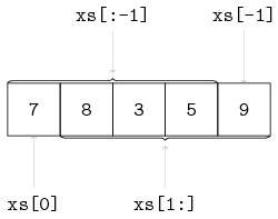
The figure below shows the two processes P and C, connected by channel variable a:
Processes are denoted by circles, and channels are denoted by directed arrows in the figure.
The arrow denotes the direction of communication.
Process P is the sender or producer, process C is the receiver or consumer.
In this case, the producer sends a finite stream of integer values (5 numbers) to the consumer. The consumer receives these values and writes them to the screen. The model is:
proc P(chan! int a):
    for i in range(5):
        a!i
    end
end

proc C(chan? int b):
    int x;

    while true:
        b?x;
        write("%d\n",x)
    end
end

model M():
    chan int a;

    run P(a), C(a)
end
The model instantiates processes P and C.
The two processes are connected to each other via channel variable a which is given as actual parameter in the run statement.
This value is copied into the local formal parameter a in process P and in formal parameter b inside process C.
Process P can send a value of type int via the actual channel parameter a to process C.
In this case P first tries to send the value 0.
Process C tries to receive a value of type int via the actual channel parameter a.
Both processes can communicate, so the communication occurs and the value 0 is sent to process C.
The received value is assigned in process C to variable x.
The value of x is printed and the cycle starts again.
This model writes the sequence 0, 1, 2, 3, 4 to the screen.
Synchronization channels
Above, process P constructs the numbers and sends them to process C.
However, since it is known that the number sequence starts at 0 and increments by one each time, there is no actual need to transfer a number.
Process C could also construct the number by itself after getting a signal (a 'go ahead') from process P.
Such signals are called synchronization signals, transfered by means of a synchronization channel.
The signal does not carry any data, it just synchronizes a send and a receive between different processes.
(Since there is no actual data transfered, the notion of sender and receiver is ambiguous.
However, in modeling there is often a notion of 'initiator' process that can be conveniently expressed with sending.)
The following example shows the use of synchronization signals between processes P and C.
The connecting channel 'transfers' values of type void.
The type void means that 'non-values' are sent and received; the type void is only allowed in combination with channels.
The iconic model is given in the previous figure, at the start of this chapter.
The model is:
proc P(chan! void a):
    for i in range(5):
        a!    # No data is being sent
    end
end

proc C(chan? void b):
    int i;

    while true:
        b?;   # Nothing is being received
        write("%d\n", i);
        i = i + 1
    end
end

model M():
    chan void a;

    run P(a), C(a)
end
Process P sends a signal (and no value is sent), and process C receives a signal (without a value).
The signal is used by process C to write the value of i and to increment variable i.
The effect of the model is identical to the previous example: the numbers 0, 1, 2, 3, 4 appear on the screen.
Two channels
A process can have more than one channel, allowing interaction with several other processes.
The next example shows two channel variables, a and b, and three processes, generator G, server S and exit E.
The iconic model is given below:
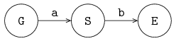
Process G is connected via channel variable a to process S and process S is connected via channel variable b to process E.
The model is:
proc G(chan! int a):
    for x in range(5):
        a!x
    end
end

proc S(chan? int a; chan! int b):
    int x;

    while true:
        a?x; x = 2 * x; b!x
    end
end

proc E(chan int a):
    int x;

    while true:
        a?x;
        write("E %d\n", x)
    end
end

model M():
    chan int a,b;

    run G(a), S(a,b), E(b)
end
The model contains two channel variables a and b.
The processes are connected to each other in model M.
The processes are instantiated and run where the formal parameters are replaced by the actual parameters.
Process G sends a stream of integer values 0, 1, 2, 3, 4 to another process via channel a.
Process S receives a value via channel a, assigns this value to variable x, doubles the value of the variable, and sends the value of the variable via b to another process.
Process E receives a value via channel b, assigns this value to the variable x, and prints this value.
The result of the model is given by:
E   0
E   2
E   4
E   6
E   8
After printing this five lines, process G stops, process S is blocked, as well as process E, the model gets blocked, and the model ends.
More senders or receivers
Channels send a message (or a signal in case of synchronization channels) from one sender to one receiver. It is however allowed to give the same channel to several sender or receiver processes. The channel selects a sender and a receiver before each communication.
The following example gives an illustration:
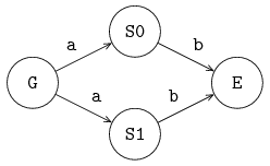
Suppose that only G and S0 want to communicate.
The channel can select a sender (namely G) and a receiver (process S0), and let both processes communicate with each other.
When sender G, and both receivers (S0 and S1), want to communicate, the channel selects a sender (G as it is the only sender available to the channel), and a receiver (either process S0 or process S1), and it lets the selected processes communicate with each other.
This selection process is non-deterministic; a choice is made, but it is unknown how the selection takes place and it cannot be influenced.
Note that a non-deterministic choice is different from a random choice.
In the latter case, there are known probabilities of selecting a process.
Sharing a channel in this way allows to send data to receiving processes where the receiving party is not relevant (either server process will do). This way of communication is different from broadcasting, where both servers receive the same data value. Broadcasting is not supported by the Chi language.
In case of two senders, S0 and S1, and one receiver E the selection process is the same.
If one of the two servers S can communicate with exit E, communication between that server and the exit takes place.
If both servers can communicate, a non-deterministic choice is made.
Having several senders and several receivers for a single channel is also handled in the same manner. A non-deterministic choice is made for the sending process and a non-deterministic choice is made for the receiving process before each communication.
To communicate with several other processes but without non-determinism, unique channels must be used.
Notes
-
The direction in channels, denoted by
?or!, may be omitted. By leaving it out, the semantics of the parameters becomes less clear (the direction of communication has to be derived from the process code). -
There are a several ways to name channels:
-
Start naming formal channel parameters in each new process with
a,b, etc. The actual names follow from the figure. This convention is followed in this chapter. For small models this convention is easy and works well, for complicated models this convention can be error-prone. -
Use the actual names of the channel parameters in the figures as formal names in the processes. Start naming in figures with
a,b, etc. This convention works well, if both figure and code are at hand during the design process. If many processes have sub-processes, this convention does not really work. -
Use unique names for the channel parameters for the whole model, and for all sub-systems, for example a channel between processes
AandBis nameda2b(the lower-case name of the sending process, followed by2, denoting 'to', and the lower-case name of the receiving process).In this case the formal and actual parameters can be in most cases the same. If many identical processes are used, this convention does not really work.
-
In the text all three conventions are used, depending on the structure of the model.
Exercises
-
Given is the specification of process
Pand modelPP:proc P(chan int a, b): int x; while true: a?x; x = x + 1; write("%d\n", x); b!x end end model PP(): chan int a, b; run P(a,b), P(b,a) end-
Study this specification.
-
Why does the model terminate immediately?
-
-
Six children have been given the assignment to perform a series of calculations on the numbers
0, 1, 2, 3, ..., 9, namely add 2, multiply by 3, multiply by 2, and add 6 subsequently. They decide to split up the calculations and to operate in parallel. They sit down at a table next to each other. The first child, the readerR, reads the numbers0, 1, 2, 3, ..., 9one by one to the first calculating childC1. ChildC1adds 2 and tells the result to its right neighbour, childC2. After telling the result to childC2, childC1is able to start calculating on the next number the readerRtells him. ChildrenC2,C3, andC4are analogous to childC1; they each perform a different calculation on a number they hear and tell the result to their right neighbor. At the end of the table the writerWwrites every result he hears down on paper. A schematic drawing of the children at the table, is given below: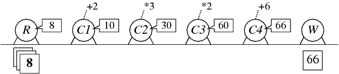
-
Finish the specification for the reading child
R, that reads the numbers 0 till 9 one by one:proc R(...): int i; while i < 10: ...; ... end end -
Specify the parameterized process
Caddthat represents the childrenC1andC4, who perform an addition. -
Specify the parameterized process
Cmulthat represents the childrenC2andC3, who perform a multiplication. -
Specify the process
Wrepresenting the writing child. Write each result to the screen separated by a new line. -
Make a graphical representation of the model
SixChildrenthat is composed of the six children. -
Specify the model
SixChildren. Simulate the model.
-
Buffers
In the previous chapter, a production system was discussed that passes values from one process to the next using channels, in a synchronous manner. (Sender and receiver perform the communication at exactly the same moment in time, and the communication is instantaneous.) In many systems however, processes do not use synchronous communication, they use asynchronous communication instead. Values (products, packets, messages, simple tokens, and so on) are sent, temporarily stored in a buffer, and then received.
In fact, the decoupling of sending and receiving is very important, it allows compensating temporarily differences between the number of items that are sent and received. (Under the assumption that the receiver is fast enough to keep up with the sender in general, otherwise the buffer will grow forever or overflow.)
For example, consider the exchange of items from a producer process P to a consumer process C as shown in the following figure:
In the unbuffered situation, both processes communicate at the same time. This means that when one process is (temporarily) faster than the other, it has to wait for the other process before communication can take place. With a buffer in-between, the producer can give its item to the buffer, and continue with its work. Likewise, the consumer can pick up a new item from the buffer at any later time (if the buffer has items).
In Chi, buffers are not modeled as channels, they are modeled as additional processes instead. The result is shown in the following figure:
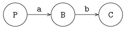
The producer sends its items synchronously (using channel a) to the buffer process.
The buffer process keeps the item until it is needed.
The consumer gets an item synchronously (using channel b) from the buffer when it needs a new item (and one is available).
In manufacturing networks, buffers, in combination with servers, play a prominent role, for buffering items in the network. Various buffer types exist in these networks: buffers can have a finite or infinite capacity, they have a input/output discipline, for example a first-out queuing discipline or a priority-based discipline. Buffers can store different kinds of items, for example, product-items, information-items, or a combination of both. Buffers may also have sorting facilities, etc.
In this chapter some buffer types are described, and with the presented concepts numerous types of buffer can be designed by the engineer. First a simple buffer process with one buffer position is presented, followed by more advanced buffer models. The producer and consumer processes are not discussed in this chapter.
A one-place buffer
A buffer usually has a receiving channel and a sending channel, for receiving and sending items.
A buffer, buffer B1, is presented in the figure below:
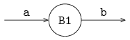
The simplest buffer is a one-place buffer, for buffering precisely one item. A one-place buffer can be defined by:
proc B1(chan? item a; chan! item b):
    item x;

    while true:
        a?x; b!x
    end
end
where a and b are the receiving and sending channels.
Item x is buffered in the process.
A buffer receives an item, stores the item, and sends the item to the next process, if the next process is willing to receive the item.
The buffer is not willing to receive a second item, as long as the first item is still in the buffer.
A two-place buffer can be created, by using the one-place buffer process twice. A two-place buffer is depicted below:
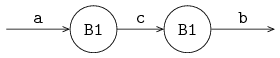
A two-place buffer is defined by:
proc B2(chan? item a; chan! item b):
    chan item c;

    run B1(a, c), B1(c, b)
end
where two processes B1 buffer maximal two items.
If each process B1 contains an item, a third item has to wait in front of process B2.
This procedure can be extended to create even larger buffers.
Another, more preferable manner however, is to describe a buffer in a single process by using a select statement and a list for storage of the items.
Such a buffer is discussed in the next section.
A single process buffer
An informal description of the process of a buffer, with an arbitrary number of stored items, is the following:
-
If the buffer has space for an item, and can receive an item from another process via channel
a, the buffer process receives that item, and stores the item in the buffer. -
If the buffer contains at least one item, and the buffer can send that item to another process via channel
b, the buffer process sends that item, and removes that item from the buffer. -
If the buffer can both send and receive a value, the buffer process selects one of the two possibilities (in a non-deterministic manner).
-
If the buffer cannot receive an item, and cannot send an item, the buffer process waits.
Next to the sending and receiving of items (to and from the buffer process) is the question of how to order the stored items. A common form is the first-in first-out (fifo) queuing discipline. Items that enter the buffer first (first-in) also leave first (first-out), the order of items is preserved by the buffer process.
In the model of the buffer, an (ordered) list of type item is used for storing the received items.
New item x is added at the rear of list xs by the statement:
xs = xs + [x]The first item of the list is sent, and then deleted with:
xs = xs[1:]An alternative solution is to swap the function of the rear and the front, which can be useful some times.
The statement to monitor several channels at the same time is the select statement.
The syntax of the select statement, with two alternatives, is:
select
    boolean_expression_1, communication statement_1:
        statement_list_1
alt
    boolean_expression_2, communication statement_2:
        statement_list_2
...
end
There has to be at least one alternative in a select statement.
The statement waits, until for one of the alternatives the boolean_expression holds and communication using the communication statement is possible.
(When there are several such alternatives, one of them is non-deterministically chosen.) For the selected alternative, the communication statement is executed, followed by the statements in the statement_list of the alternative.
The above syntax is the most generic form, the boolean_expression may be omitted when it always holds, or the communication statement may be omitted when there is no need to communicate.
The , also disappears then.
(Omitting both the boolean expression and the communication statement is not allowed.) Similarly, when the statement_list is empty or just pass, it may be omitted (together with the : in front of it).
The description (in words) of the core of the buffer, from the start of this section, is translated in code, by using a select statement:
select
    size(xs) < N, a?x:
        xs = xs + [x]
alt
    size(xs) > 0, b!xs[0]:
        xs = xs[1:]
end
In the first alternative, it is stated that, if the buffer is not full, and the buffer can receive an item, an item is received, and that item is added to the rear of the list. In the second alternative, it is stated that, if the buffer contains at least one item, and the buffer can send an item, the first item in the list is sent, and the list is updated. Please keep in mind that both the condition must hold and the communication must be possible at the same moment.
The complete description of the buffer is:
proc B(chan? item a; chan! item b):
    list item xs; item x;

    while true:
        select
            size(xs) < N, a?x:
                xs = xs + [x]
        alt
            size(xs) > 0, b!xs[0]:
                xs = xs[1:]
        end
    end
end
Instead of boolean expression size(xs) > 0, expression not empty(xs) can be used, where empty is a function yielding true if the list is empty, otherwise false.
In case the capacity of the buffer is infinite, expression size(xs) < N can be replaced by true, or even omitted (including the comma).
An infinite buffer
A buffer with infinite capacity can be written as:
proc B(chan? item a; chan! item b):
    list item xs; item x;

    while true:
        select
            a?x:
                xs = xs + [x]
        alt
            not empty(xs), b!xs[0]:
                xs = xs[1:]
        end
    end
end
A first-in first-out buffer is also called a queue, while a first-in last-out buffer (lifo buffer), is called a stack. A description of a lifo buffer is:
proc B(chan? item a; chan! item b):
    list item xs; item x;

    while true:
        select
            a?x:
                xs = [x] + xs
        alt
            not empty(xs), b!xs[0]:
                xs = xs[1:]
        end
    end
end
The buffer puts the last received item at the head of the list, and gets the first item from the list. An alternative is to put the last item at the rear of the list, and to get the last item from the list.
A token buffer
In the next example, signals are buffered instead of items.
The buffer receives and sends 'empty' items or tokens.
Counter variable w of type int denotes the difference between the number of tokens received and the number of tokens sent.
If the buffer receives a token, counter w is incremented; if the buffer sends a token, counter w is decremented.
If the number of tokens sent is less than the number of tokens received, there are tokens in the buffer, and w > 0.
A receiving channel variable a of type void is defined for receiving tokens.
A sending channel variable b of type void is defined for sending tokens.
The buffer becomes:
proc B(chan? void a; chan! void b):
    int w;

    while true:
        select
            a?:
                w = w + 1
        alt
            w > 0, b!:
                w = w - 1
        end
    end
end
Note that variables of type void do not exist.
Type void only can be used in combination with channels.
A priority buffer
A buffer for items with different priority is described in this section. An item has a high priority or a normal priority. Items with a high priority should leave the buffer first.
An item is a tuple with a field prio, denoting the priority, 0 for high priority, and 1 for normal priority:
type item = tuple(...; int prio);For the storage of items, two lists are used: a list for high priority items and a list for normal priority items. The two lists are described by a list with size two:
list(2) list item xs;Variable xs[0] contains the high priority items, xs[1] the normal priority items.
The first item in the high priority list is denoted by xs[0][0], etc.
In the model the received items are, on the basis of the value of the prio-field in the item, stored in one of the two lists: one list for 'high' items and one list for 'normal' items.
The discipline of the buffer is that items with a high priority leave the buffer first.
The model is:
proc BPrio(chan? item a; chan! item b):
    list(2) list item xs; item x;

    while true:
        select
            a?x:
                xs[x.prio] = xs[x.prio] + [x]
        alt
            not empty(xs[0]), b!xs[0][0]:
                xs[0] = xs[0][1:]
        alt
            empty(xs[0]) and not empty(xs[1]), b!xs[1][0]:
                xs[1] = xs[1][1:]
        end
    end
end
The buffer has two lists xs[0] and xs[1].
Received items x are stored in xs[x.prio] by the statement xs[x.prio] = xs[x.prio] + [x].
If the list high priority items (xs[0]) is not empty, items with high priority are sent.
The first element in list xs[0] is element xs[0][0].
If there are no high priority items (list xs[0] is empty), and there are normal priority items (list xs[1] is not empty), the first element of list xs[1], element xs[1][0], is sent.
Note that the order of the alternatives in the select statement does not matter, every alternative is treated in the same way.
Exercises
-
To study product flow to and from a factory, a setup as shown in the figure below is created:
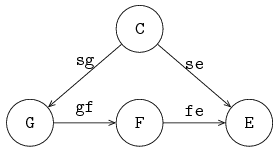
Fis the factory being studied, generatorGsends products into the factory, and exit processEretrieves finished products. The factory is tightly controlled by controllerCthat sends a signal toGorEbefore a product may be moved. The model is as follows:proc G(chan! int a; chan? void sg): for i in range(10): sg?; a!i; end end proc F(chan? int a; chan! int b): ... end proc E(chan? int a; chan? void se): int x; while true: se?; a?x; write("E received %d\n", x); end end proc C(chan! void sg, se; int low, high): int count; while true: while count < high: sg!; count = count + 1; end while count > low: se!; count = count - 1; end end end model M(): chan void sg, se; chan int gf, fe; run C(sg, se, 0, 1), G(gf, sg), F(gf, fe), E(fe, se); endThe number of products inserted by the generator has been limited to allow for manual inspection of results.
-
As a model of the factory, use a FIFO buffer process. Run the simulation, and check whether all products are received by the exit process.
-
Change the control policy to
low = 1andhigh = 4. Predict the outcome, and verify with simulation. -
The employees of the factory propose to stack the products in the factory to reduce the amount of space needed for buffering. Replace the factory process with a LIFO buffer process, run the experiments again, first with
low = 0andhigh = 1and then withlow = 1andhigh = 4. -
You will notice that some products stay in the factory forever. Why does that happen? How should the policy be changed to ensure all products eventually leave the factory?
-
Servers with time
A manufacturing line contains machines and/or persons that perform a sequence of tasks, where each machine or person is responsible for a single task. The term server is used for a machine or a person that performs a task. Usually the execution of a task takes time, e.g. a drilling process, a welding process, the set-up of a machine. In this chapter we introduce the concept of time, together with the delay statement.
Note that here 'time' means the simulated time inside the model. For example, assume there are two tasks that have to be performed in sequence in the modeled system. The first task takes three hours to complete, the second task takes five hours to complete. These amounts of time are specified in the model (using the delay statement, as will be explained below). A simulation of the system should report 'It takes eight hours from start of the first task to finish of the second task'. However, it generally does not take eight hours to compute that result, a computer can calculate the answer much faster. When an engineer says ''I had to run the system for a year to reach steady-state'', he means that time inside the model has progressed a year.
The clock
The variable time denotes the current time in a model.
It is a global variable, it can be used in every model and proc.
The time is a variable of type real.
Its initial value is 0.0.
The variable is updated automatically by the model, it cannot be changed by the user.
The unit of the time is however determined by the user, that is, you define how long 1 time unit of simulated time is in the model.
The value of variable time can be retrieved by reading from the time variable:
t = timeThe meaning of this statement is that the current time is copied to variable t of type real.
A process delays itself to simulate the processing time of an operation with a delay statement. The process postpones or suspends its own actions until the delay ends.
For example, suppose a system has to perform three actions, each action takes 45 seconds. The unit of time in the model is one minute (that is, progress of the modeled time by one time unit means a minute of simulated time has passed). The model looks like:
proc P():
    for i in range(3):
        write("i = %d, time = %f\n", i, time);
        delay 0.75
    end
end

model M():
    run P()
end
An action takes 45 seconds, which is 0.75 time units.
The delay 0.75 statement represents performing the action, the process is suspended until 0.75 units of time has passed.
The simulation reports:
i = 0, time = 0.000000
i = 1, time = 0.750000
i = 2, time = 1.500000
All processes finished at time 2.25
The three actions are done in 2.25 time units (2.25 minutes).
Adding time
Adding time to the model allows answering questions about time, often performance questions ('how many products can I make in this situation?'). Two things are needed:
-
Servers must model use of time to perform their task.
-
The model must perform measurements of how much time passes.
By extending models of the servers with time, time passes while tasks are being performed. Time measurements then give non-zero numbers (servers that can perform actions instantly result in all tasks being done in one moment of time, that is 0 time units have passed between start and finish). Careful analysis of the measurements should yields answers to questions about performance.
In this chapter, adding of passing time in a server and how to embed time measurements in the model is explained. The first case is a small production line with a deterministic server (its task takes a fixed amount of time), while the second case uses stochastic arrivals (the moment of arrival of new items varies), and a stochastic server instead (the duration of the task varies each time). In both cases, the question is what the flow time of an item is (the amount of time that a single item is in the system), and what the throughput of the entire system is (the number of items the production line can manufacture per time unit).
A deterministic system
The model of a deterministic system consists of a deterministic generator, a deterministic server, and an exit process. The line is depicted in the following figure:
Generator process G sends items, with constant inter-arrival time ta, via channel a, to server process S.
The server processes items with constant processing time ts, and sends items, via channel b, to exit process E.
An item contains a real value, denoting the creation time of the item, for calculating the throughput of the system and flow time (or sojourn time) of an item in the system.
The generator process creates an item (and sets its creation time), the exit process E writes the measurements (the moment in time when the item arrives in the exit process, and its creation time) to the output.
From these measurements, throughput and flow time can be calculated.
Model M describes the system:
type item = real;

model M(real ta, ts; int N):
    chan item a, b;

    run G(a, ta),
        S(a, b, ts),
        E(b, N)
end
The item is a real number for storing the creation time.
Parameter ta denotes the inter-arrival time, and is used in generator G.
Parameter ts denotes the server processing time, and is used in server S.
Parameter N denotes the number of items that must flow through the system to get a good measurement.
Generator G has two parameters, channel a, and inter-arrival time ta.
The description of process G is given by:
proc G(chan! item a; real ta):
    while true:
        a!time; delay ta
    end
end
Process G sends an item, with the current time, and delays for ta, before sending the next item to server process S.
Server S has three parameters, receiving channel a, sending channel b, and server processing time ts:
proc S(chan? item a; chan! item b; real ts):
    item x;

    while true:
        a?x; delay ts; b!x
    end
end
The process receives an item from process G, processes the item during ts time units, and sends the item to exit process E.
Exit E has two parameters, receiving channel a and the length of the experiment N:
proc E(chan item a; int N):
    item x;

    for i in range(N):
        a?x; write("%f, %f\n", time, time - x)
    end
end
The process writes current time time and item flow time time - x to the screen for each received item.
Analysis of the measurements will show that the system throughput equals 1 / ta, and that the item flow time equals ts (if ta >= ts).
A stochastic system
In the next model, the generator produces items with an exponential inter-arrival time, and the server processes items with an exponential server processing time. To compensate for the variations in time of the generator and the server, a buffer process has been added. The model is depicted below:
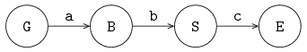
Type item is the same as in the previous situation.
The model runs the additional buffer process:
model M(real ta, ts; int N):
    chan item a, b, c;

    run G(a, ta),
        B(a, b),
        S(b, c, ts),
        E(c, N)
end
Generator G has two parameters, channel variable a, and variable ta, denoting the mean inter-arrival time.
An exponential distribution is used for deciding the inter-arrival time of new items:
proc G(chan item a; real ta):
    dist real u = exponential(ta);

    while true:
        a!time; delay sample u
    end
end
The process sends a new item to the buffer, and delays sample u time units.
Buffer process B is a fifo buffer with infinite capacity, as described at An infinite buffer.
Server S has three parameters, channel variables a and b, for receiving and sending items, and a variable for the average processing time ts:
proc S(chan item a, b; real ts):
    dist real u = exponential(ts);
    item x;

    while true:
        a?x; delay sample u; b!x
    end
end
An exponential distribution is used for deciding the processing time.
The process receives an item from process G, processes the item during sample u time units, and sends the item to exit process E.
Exit process E is the same as previously, see A deterministic system.
In this case the throughput of the system also equals 1 / ta, and the mean flow can be obtained by doing an experiment and analysis of the resulting measurements (for ta > ts).
Two servers
In this section two different types of systems are shown: a serial and a parallel system. In a serial system the servers are positioned after each other, in a parallel system the servers are operating in parallel. Both systems use a stochastic generator, and stochastic servers.
Serial system
The next model describes a serial system, where an item is processed by one server, followed by another server. The generator and the servers are decoupled by buffers. The model is depicted below:
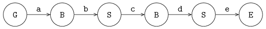
The model can be described by:
model M(real ta, ts; int N):
    chan item a, b, c, d, e;

    run G(a, ta),
        B(a, b), S(b, c, ts),
        B(c, d), S(d, e, ts),
        E(e, N)
end
The various processes are equal to those described previously in A stochastic system.
Parallel systems
In a parallel system the servers are operating in parallel. Having several servers in parallel is useful for enlarging the processing capacity of the task being done, or for reducing the effect of break downs of servers (when a server breaks down, the other server continues with the task for other items). The system is depicted below:
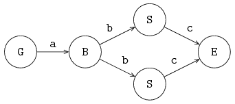
Generator process G sends items via a to buffer process B, and process B sends the items in a first-in first-out manner to the servers S.
Both servers send the processed items to the exit process E via channel c.
The inter-arrival time and the two process times are assumed to be stochastic, and exponentially distributed.
Items can pass each other, due to differences in processing time between the two servers.
If a server is free, and the buffer is not empty, an item is sent to a server. If both servers are free, one server will get the item, but which one cannot be determined beforehand. (How long a server has been idle is not taken into account.) The model is described by:
model M(real ta, ts; int N):
    chan item a, b, c;

    run G(a, ta),
        B(a, b),
        S(b, c, ts), S(b, c, ts),
        E(c, N)
end
To control which server gets the next item, each server must have its own channel from the buffer. In addition, the buffer has to know when the server can receive a new item. The latter is done with a 'request' channel, denoting that a server is free and needs a new item. The server sends its own identity as request, the requests are administrated in the buffer. The model is depicted below:
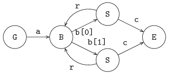
In this model, the servers 'pull' an item through the line. The model is:
model M(real ta, ts; int N):
    chan item a; list(2) chan item b; chan item c;
    chan int r;

    run G(a, ta),
        B(a, b, r),
        unwind j in range(2):
            S(b[j], c, r, ts, j)
        end,
        E(c, N)
end
In this model, an unwind statement is used for the initialization and running of the two servers.
Via channel r an integer value, 0 or 1, is sent to the buffer.
The items received from generator G are stored in list xs, the requests received from the servers are stored in list ys.
The items and requests are removed form their respective lists in a first-in first-out manner.
Process B is defined by:
proc B(chan? item a; list chan! item b; chan? int r):
    list item xs; item x;
    list int ys; int y;

    while true:
        select
            a?x:
                xs = xs + [x]
        alt
            r?y:
                ys = ys + [y]
        alt
            not empty(xs) and not empty(ys), b[ys[0]]!xs[0]:
                xs = xs[1:]; ys = ys[1:]
        end
    end
end
If, there is an item present, and there is a server demanding for an item, the process sends the first item to the longest waiting server.
The longest waiting server is denoted by variable ys[0].
The head of the item list is denoted by xs[0].
Assume the value of ys[0] equals 1, then the expression b[ys[0]]!xs[0], equals b[1]!xs[0], indicates that the first item of list xs, equals xs[0], is sent to server 1.
The server first sends a request via channel r to the buffer, and waits for an item.
The item is processed, and sent to exit process E:
proc S(chan? item b; chan! item c; chan! int r; real ts; int k):
    dist real u = exponential(ts);
    item x;

    while true:
        r!k;
        b?x;
        delay sample u;
        c!x
    end
end
Assembly
In assembly systems, components are assembled into bigger components. These bigger components are assembled into even bigger components. In this way, products are built, e.g. tables, chairs, computers, or cars. In this section some simple assembly processes are described. These systems illustrate how assembling can be performed: in industry these assembly processes are often more complicated.
An assembly work station for two components is shown below:
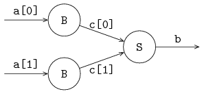
The assembly process server S is preceded by buffers.
The server receives an item from each buffer B, before starting assembly.
The received items are assembled into one new item, a list of its (sub-)items.
The description of the assembly server is:
proc S(list chan? item c, chan! list item b):
    list(2) item v;

    while true:
        select
            c[0]?v[0]: c[1]?v[1]
        alt
            c[1]?v[1]: c[0]?v[0]
        end
        b!v
    end
end
The process takes a list of channels c to receive items from the preceding buffers.
The output channel b is used to send the assembled component away to the next process.
First, the assembly process receives an item from both buffers.
All buffers are queried at the same time, since it is unknown which buffer has components available.
If the first buffer reacts first, and sends an item, it is received with channel c[0] and stored in v[0] in the first alternative.
The next step is then to receive the second component from the second buffer, and store it (c[1]?v[1]).
The second alternative does the same, but with the channels and stored items swapped.
When both components have been received, the assembled product is sent away.
A generalized assembly work station for n components is depicted below.
In the figure, m = n - 1.
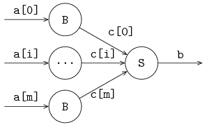
The entire work station (the combined buffer processes and the assembly server process) is described by:
proc W(list chan? item a; chan! list item b):
    list(size(a)) chan item c;

    run unwind i in range(size(a)):
            B(a[i], c[i])
        end,
        S(c,b)
end
The size of the list of channels a is determined during initialization of the workstation.
This size is used for the generation of the process buffers, and the accompanying channels.
The assembly server process works in the same way as before, except for a generic n components, it is impossible to write a select statement explicitly.
Instead, an unwind is used to unfold the alternatives:
proc S(list chan? item c, chan! list item b):
    list(size(c)) item v;
    list int rec;

    while true:
        rec = range(size(c));
        while not empty(rec):
            select
                unwind i in rec
                    c[i]?v[i]: rec = rec - [i]
                end
            end
        end;
        delay ...;
        b!v
    end
end
The received components are again in v.
Item v[i] is received from channel c[i].
The indices of the channels that have not provided an item are in the list rec.
Initially, it contains all channels 0 … size(c), that is, range(size(c)).
While rec still has a channel index to monitor, the unwind i in rec unfolds all alternatives that are in the list.
For example, if rec contains [0, 1, 5], the select unwind i in rec ... end is equivalent to:
select
    c[0]?v[0]: rec = rec - [0]
alt
    c[1]?v[1]: rec = rec - [1]
alt
    c[5]?v[5]: rec = rec - [5]
end
After receiving an item, the index of the channel is removed from rec to prevent receiving a second item from the same channel.
When all items have been received, the assembly process starts (modeled with a delay, followed by sending the assembled component away with b!v.
In practical situations these assembly processes are performed in a more cascading manner. Two or three components are 'glued' together in one assemble process, followed in the next process by another assembly process.
Exercises
-
To understand how time and time units relate to each other, change the time unit of the model in The clock.
-
Change the model to using time units of one second (that is, one time unit means one second of simulated time).
-
Predict the resulting throughput and flow time for a deterministic case like in Adding time, with
ta = 4andts = 5. Verify the prediction with an experiment, and explain the result.
-
-
Extend the model A controlled factory in Buffer exercises with a single deterministic server taking
4.0time units to model the production capacity of the factory. Increase the number of products inserted by the generator, and measure the average flow time for-
A FIFO buffer with control policy
low = 0andhigh = 1. -
A FIFO buffer with control policy
low = 1andhigh = 4. -
A LIFO buffer with control policy
low = 1andhigh = 4.
-
Conveyors
A conveyor is a long belt on which items are placed at the starting point of the conveyor. The items leave the conveyor at the end point, after traveling a certain period of time on the conveyor. The number of items traveling on the conveyor varies, while each item stays the same amount of time on the conveyor. It works like a buffer that provides output based on item arrival time instead of based on demand from the next process.
Timers
To model a conveyor, you have to wait until a particular point in time.
The Chi language has timers to signal such a time-out.
The timer is started by assigning it a value.
From that moment, it automatically decrements when time progresses in the model, until it reaches zero.
The function ready gives the boolean value true if the timer is ready.
The amount of time left can be obtained by reading from the variable.
An example:
proc P():
    timer t;

    delay 10.0;
    t = timer(5.0); # Get a time-out at time = 15.0
    for i in range(7):
        write("%f %f %b\n", time, real(t), ready(t));
        delay 1.0
    end
end

model M():
    run P()
end
Initially, time equals 0.0.
The first action of process P is to delay the time for 10.0 time units.
Now the value of time equals 10.0.
Nothing happens to timer t as it was already zero.
At time 10 timer t is started with the value 5.0.
The output of the program is:
10.0   5.0    false
11.0   4.0    false
12.0   3.0    false
13.0   2.0    false
14.0   1.0    false
15.0   0.0    true
16.0   0.0    true
Timer t decrements as time progresses, and it is ready at 10.0 + 5.0 units.
A process can have more timers active at the same moment.
A conveyor
A conveyor is schematically depicted in the following figure:
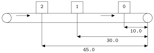
Three items are placed on the conveyor.
For simplicity, assume the conveyor is 60.0 meter long and has a speed of 1 meter per second.
An item thus stays on the conveyor for 60.0 seconds.
Item 0 has been placed on the conveyor 50.0 seconds ago, and will leave the conveyor 10.0 second from now.
In the same way, item 1 will leave 30.0 seconds from now, and 2 leaves after 45.0 seconds.
Each item has a yellow sticker with the time that the item leaves the conveyor.
Based on this idea, tuple type conv_item has been defined, consisting of a field item, denoting the received item, and a timer field t, with the remaining time until the item leaves the conveyor:
type conv_item = tuple(item x; timer t);

proc T(chan? item a; chan! item b; real convey_time):
    list conv_item xst; item x;

    while true:
        select
            a?x:
                xst = xst + [(x, timer(convey_time))]
        alt
            not empty(xst) and ready(xst[0].t), b!xst[0].x:
                xst = xst[1:]
        end
    end
end
The conveyor always accepts new items from channel a, and adds the item with the yellow sticker to the list.
If the conveyor is not empty, and the timer has expired for the first item in the list, it is sent (without sticker) to the next process.
The conveyor sends items to a process that is always willing to a receive an item, this implies that the conveyor is never blocked.
Blocking implies that the items nevertheless are transported to the end of the conveyor.
A priority conveyor
In this example, items are placed on a conveyor, where the time of an item on the conveyor varies between items.
Items arriving at the conveyor process, get inserted in the list with waiting items, in ascending order of their remaining time on the conveyor.
The field tt in the item denotes the traveling time of the item on the conveyor:
type item      = tuple(...; real tt; ...),
     conv_item = tuple(item x; timer t);
The predicate function pred is defined by:
func bool pred(conv_item x, y):
    return real(x.t) <= real(y.t)
end
The conveyor process becomes:
proc T(chan? item a; chan! item b):
    list conv_item xst; item x;

    while true:
        select
            a?x:
                xst = insert(xst, (x, timer(x.tt)), pred)
        alt
            not empty(xst) and ready(xst[0].t), b!xst[0].item:
                xst = xst[1:]
        end
    end
end
The conveyor process works like before, except the new item is inserted in the list according to its remaining time, instead of at the rear of the list.
Exercises
-
Model the system as shown in the figure below, where
Tis a conveyor process with a capacity of at most three products and exponentially distributed conveying times with an average of4.0.Compute the average flow time of products in the system.
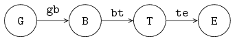
-
Model the system as shown in the figure below, with exponentially distributed server processing times with an average of
4.0.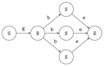
-
Compute the average flow time of products in the system.
-
Are there differences in behavior between both systems? Why (not)?
-
Simulations and experiments
So far, attention has focused on the Chi language, and how to use it for modeling a discrete-event system.
In this chapter, the focus shifts to performing simulations, in particular for systems with infinite behavior. Also, how to perform multiple model simulations is explained.
Simulating finite systems
For systems that have simple cyclic behavior, the simulation can be 'exhaustive', for example:
proc G(chan! real a):
    a!time
end

proc M(chan? real a, chan! real b):
    real x;

    a?x; delay 5.0; b!x
end

proc E(chan? real a):
    real x;

    a?x;
    writeln("Flow time: %.2f", time - x);
end

model M():
    chan real gm, me;

    run G(gm), M(gm, me), E(me);
end
This simulation sends a single product through the line, prints the flow time, and exits.
(All processes end, which makes that the run statement and the model end as well.)
In this case, the answer is even obvious without running the simulation.
Simulating infinite systems
For other systems, it is much harder to decide when enough has been simulated.
Typically, a process (E in the example below), collects values of the property of interest (for example flow time of products), until it has collected enough samples to draw a conclusion, and compute the resulting value.
After doing so, the problem arises to let all processes know the simulation should be stopped.
This can be programmed in the model (such as adding channels to signal termination of the simulation to all processes).
A simpler alternative is to use the exit statement, in the following way:
proc real E(chan? real a, int N):
    real total, x;

    for n in range(N):
        a?x;
        total = total + time - x;
    end;
    exit total / N
end

model real M(... int N):
    ...

    run ..., E(..., N);
end
In process E, the average flow time is calculated and given as argument of the exit statement.
At the moment this statement is executed, the model and all processes are killed, and the computed value becomes the exit value (the result) of the simulation.
The real type before the name E denotes that the process may perform an exit statement returning a real value.
The model runs the E process, so it may also give an exit value as result.
These types are called exit type.
Exit values are printed to the screen by the simulator when it ends the model simulation.
Another option is to use write to output the computed value, and use exit without argument.
In that case, the exit value is of type void.
Simulating several scenarios
The above works nicely for single model simulations. The model is started one time, and it derives a result for a single scenario.
Often however, you want to perform several model simulations. This can be the exact same scenario when the model has stochastic behavior, or it can be with different parameter values each time (to investigate system behavior under different circumstances). In such cases, you can use an experiment, like below:
xper X():
    real v;
    int n;

    for n in range(5, 10):
        v = M(n);
        write("%2d: %.2f\n", n, v)
    end
end
The experiment X looks just like a function, except that it has no return statement.
It can however 'call' a model like a function.
In the example above M(n) starts a simulation with model M and the given value for n.
When the model exits by means of the exit statement (this is required!), the computed exit value of the (model) simulation is assigned to variable v.
In the experiment, this value can be used for post-processing, or in this case, get printed as result value in a table.
SVG visualization
A Chi simulation often produces large amounts of textual output that you have to process in order to understand the simulation result. Also for people unfamiliar with the details of the simulated system, results are hard to understand. A possible solution is to add a visualization of the system to the simulator, that displays how the system behaves over time. Generally, it looses some of the details, but it makes globally checking, and explaining of the simulation much easier.
The SVG file format
The Scalable Vector Graphics (SVG) file format is a widely used, royalty-free standard for two-dimensional vector graphics, developed by the World Wide Web Consortium (W3C). SVG images consist of three types of objects: vector graphic shapes (rectangles, circles, etc.), raster images, and text. The benefit of vector images formats over raster image formats, is that raster images are created with a fixed size, while vector images contain a description of the image and can be rendered at any size without loss of quality.
SVG image files are stored in an XML-based file format. This means that they can be edited with any text editor. However, it is often more convenient to edit them with a drawing program that supports vector graphics, such as Adobe Illustrator or Inkscape. Most modern web browsers also support display of SVG images.
Visualization
An SVG file has a tree structure; (graphical) elements are drawn in the same order as they appear in the file. Elements further down in the file are thus drawn on top of earlier elements. Also, each element has a position and size. They may have other properties like a color or a gradient as well. There are also 'administrative' elements, that can group, scale, or rotate parts of the tree. The website of Jakob Jenkov has a very nice SVG Tutorial.
The SVG visualization by the Chi simulator exploits this structure. You access the elements, and literally change the value of their properties or copy part of the tree. The Apache Batik SVG Toolkit used for drawing the SVG image at the screen notices the changes, and updates the displayed image.
By updating the SVG tree every time when the state of the simulation changes, you can display how a system evolves over time as an animated image.
SVG visualization example
To illustrate how to make an SVG visualization, a simple generator, buffer, server, buffer, server, exit (GBSBSE) process line is used. Below the generator and exit process definitions, and the model:
proc G(chan! real to; real ptime):
    int n = 0;

    while n < 100:
        to!time; delay ptime; n = n + 1
    end
end

proc E(chan? real from):
    real x;

    while true:
        from?x
    end
end

model M():
    list(3) chan real c;
    list(2) chan real bs;

    run G(c[0], 1.1),

        B(0, c[0], bs[0], 3),
        S(0, bs[0], c[1], 1.0, exponential(10.0), exponential(4.0)),

        B(1, c[1], bs[1], 3),
        S(1, bs[1], c[2], 0.9, exponential(10.0), exponential(4.0)),

        E(c[2]);
end
This system should be visualized, where the number of items in each buffer should be displayed, and the state of each server (waiting for input, processing, or waiting for output) should also be shown. The gbse.svg SVG file was made for this purpose, which looks like
in an editor. The black rectangle represents the displayed area when the visualization is running. It has two light-green rectangles in it, representing the first and second buffer. The darker green rectangles inside will vary in height to show the number of items in each buffer.
The circle at the left of the displayed area is never displayed in the visualization. However, each server makes a copy of it, and places it at an appropriate position in the display. While for two servers, one could just as well perform the copying beforehand, as was done with the buffer graphics, but the copying technique demonstrates how to scale visualizations for displaying a larger number of items without a lot of effort.
Buffer visualization
The left darker green rectangle has an id with value buf0, while the right rectangle has an id containing buf1.
Through the id, you can access the properties, in this case, the height, for example attr buf0.height = 50.
This will set the height property of the SVG element named buf0 to 50.
The SVG visualization is not in the Chi model itself, it is an external entity. You access it by opening a 'file', and writing the commands such as above, as lines of text. The code of the buffer is shown below.
proc B(int num; chan? real from; chan! real to; int cap):
    list real xs;
    real x;
    file f = open("SVG:gbse.svg", "w");

    while true:
        select size(xs) > 0, to!xs[0]:
            xs = xs[1:];
        alt size(xs) < cap, from?x:
            xs = xs + [x]
        end
        writeln(f, "attr buf%d.height = %d", num, size(xs) * 50);
    end
    close(f);
end
It is a normal finite buffer process, except for three additional lines.
The first change is the file f = open("SVG:gbse.svg", "w"); line.
It creates a connection to the SVG visualization due to the SVG: prefix of the file name.
gbse.svg is the name of the .svg file described above.
The 'file' should be opened for writing (since you will be sending commands to it).
The second line is the writeln(f, "attr buf%d.height = %d", num, size(xs) * 50); line, which constructs a line of text to set the height of the darker green rectangle to a value proportional to the number of elements in the buffer.
There is however a vertical coordinate trick needed to make it all work.
The third line is the close(f); line at the end of the process.
It closes the connection to the SVG visualization.
Vertical coordinates trickery
In SVG, the vertical coordinates run from the top of the screen to the bottom.
If you just draw a rectangle, its base position (x,y) is at the top-left corner, with width going to the right of the screen, and height towards the bottom.
In other words, if you change the height of a simple SVG rectangle by a program like the buffer process, the rectangle will grow downwards instead of upwards!
To make it grow upwards instead, you can
-
change both the
heightand theycoordinate of the rectangle at the same time (you move the top of the rectangle in opposite direction with its growth in height, so it looks like the rectangle grows upwards), or -
flip the coordinate system of the rectangle by inserting a '180 degrees rotation' transformation around the rectangle (you tell SVG to draw the rectangle 'upside down', thus if you make it higher, it grows downwards, but the flipped coordinate displays it as growth upwards.
Server process
The server process code looks as follows (ignore all the writeln lines for now).
proc S(int num; chan? real from; chan! real to; real ptime; dist real up, down):
    real event, x;
    file f = open("SVG:gbse.svg", "w");

    writeln(f, "copy server, , _x%d", num);
    writeln(f, "absmove s_x%d (%d, 325)", num, num*420+150);

    while true:
        event = time + sample up;

        # Up; process items.
        while event > time:
            writeln(f, "attr s_x%d.fill=yellow", num);
            from?x;
            writeln(f, "attr s_x%d.fill=green", num);
            delay ptime;
            writeln(f, "attr s_x%d.fill=magenta", num);
            to!x;
        end

        # Down; repair machine.
        writeln(f, "attr s_x%d.fill=red", num);
        delay sample down;
    end
    close(f);
end
The server runs forever, starting with sampling how long it will be up (event = time + sample up).
Until it has reached that time (while event > time:), it cycles through getting a product, processing it for uptime time units, and sending the product out again.
After a few cycles, it has reached the event time, goes down, and waits for repair (delay sample down;).
Once the machine is repaired it starts again.
Visualization of the servers is discussed below.
Visualizing the server
A server is to be visualized with a circle that changes color depending on what the server is doing. Yellow means it is waiting for a product, green means processing, magenta means it is waiting to pass the finished product to the next station, and red means the machine is down. After repairing, it will continue processing.
As with the buffer process, the SVG visualization first opens a file connection to the visualizer and the SVG file with the file f = open("SVG:gbse.svg", "w"); line.
The filename of the .svg file must be the same as with the buffer process (the visualizer can only show one SVG file at a time).
To display server state in the SVG visualization, we need a circle (called arc in SVG) named s_0 and s_1 (for server 0 and server 1), positioned behind its buffer.
If there are not too many servers, and their number is fixed, one could simply add those arcs to the SVG file and be done with it.
However, if you have a lot of servers, or you don’t know in advance how many you will have, you cannot add them beforehand, you need to construct the SVG elements 'on the fly'.
Copying SVG elements
For showing the server states, arcs named s_0 and s_1 are required in SVG, which are created by copying and moving an SVG element.
In this case, a server is represented by just one SVG element, so you can copy and move that one element.
In general however, you want to copy several elements at the same time (for example you might want to copy graphical elements to display a work station, a server with its buffer).
SVG has group elements, where you can put any number of (graphical) elements inside.
When you copy a group, you copy its entire contents.
The gbse.svg file as a group called server, containing an arc element called s.
The server group is copied and moved, which causes the arc element to be copied and moved as well.
Inside an SVG file, each element must have a unique id, that is, each element must have a unique name.
When making a copy, the copied elements must thus also be given a new name.
The entire operation is performed with sending a copy [node], [prefix], [suffix] command to the SVG visualizer.
It takes the element named [node], and makes a full copy of it (all elements inside it are also copied).
For each copied element the [prefix] is added in front of its id name, and the [suffix] is added behind it.
The writeln(f, "copy server, , _x%d", num); line in the Chi simulation performs the copy operation for the servers.
It takes the server group element (which contains an s arc element), and adds nothing in front of the names (there is no text between the first and the second comma).
It appends the names with _x0 for the first server, and _x1 for the second server.
The result is thus a copy of the server group, called server_x0 or server_x1, containing an arc s_x0 respectively s_x1.
Note that the copy command performs copying, and nothing else. Since the copied element is exactly at the same position as the original, you don’t see copies. This is however fixed by a move command explained next.
Moving SVG elements
You often want to position an SVG element at some point in the display.
The simplest way to do that is to change its x and y attributes, much like the height attribute of the buffer rectangle was modified.
Another solution is to perform a relative move, using transform/translate.
This works, until you add a transformation element that changes the coordinate system. Sometimes you do this consciously, for example adding a 'flip' transformation to fix the vertical coordinates. At other times the SVG editor may insert one, for example when you rotate or scale some part of the drawing.
The Chi SVG visualizer has a absmove [node] ([xpos], [ypos]) command to handle this case.
It computes a transformation to get the top-left corner of the element named [node] at position ([xpos], [ypos]).
Keep in mind that the vertical coordinate starts at the top, and goes down.
There are limitations to this command, in some case it may fail (see the reference manual for details about the command).
It is recommended to use this command one time on an element to move it to a known base position.
Once it is at a known position, change the x and y coordinates of a child element (to avoid disturbing the base position), to move relative to that base position.
Another solution is to perform a relative move, using transform/translate.
In the Chi simulation, the writeln(f, "absmove s_x%d (%d, 325)", num, num*420+150); line moves the copied s_x0 and s_x1 arcs to the right position in the display.
With the arcs in the right position in the display, the servers can display their activities by changing the color of the fill attribute.
Chi Reference Manual
This manual explains the allowed Chi language constructs and their semantics. Topics discussed here are:
Global definitions
At global level, a Chi program is a sequence of definitions, as shown in the following diagram.
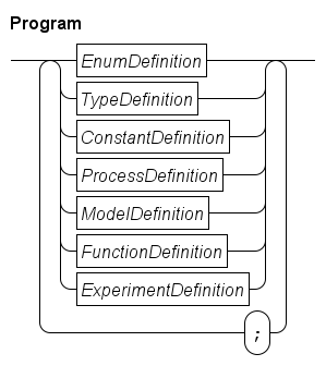
Each of the definitions is explained below.
The syntax diagram suggests that a ; separator is obligatory between definitions.
The implementation is more liberal, you may omit the separator when a definition ends with the end keyword.
Also, it is allowed to use a separator after the last definition.
The name of each global definition has to be unique.
Enumeration definitions
With enumerations, you create a new enumeration type containing a number of names (called enumeration values). The syntax is given below.
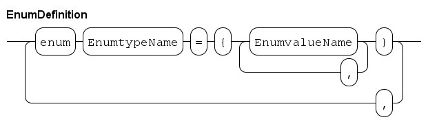
The enumeration definitions start with the keyword enum, followed by a sequence of definitions separated with a ,.
Each definition associates an enumeration type name with a set of enumeration value names.
For example:
enum FlagColours  = {red, white, blue},
     MachineState = {idle, heating, processing};
The enumeration type names act as normal types, and the enumeration values are its values. The values have to be unique words.
For example, you can create a variable, and compare values like:
MachineState state = idle;
...
while state != processing:
    ...
end
Note that enumeration values have no order, you cannot increment or decrement variables with an enumeration type, and you can only compare values with equality and inequality.
Type definitions
Type definitions allow you to assign a name to a type. By using a name instead of the type itself, readability of the program increases.
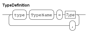
A type definition starts with the keyword type, followed by a number of 'assignments' that associate a type name with a type, separated with a ,.
For further details about type names and types, see Types.
An example:
type lot   = real,
     batch = list lot;
Here a lot type name is introduced that is implemented with a real number, and a batch type name is created, which is a list of lot.
These type names can be used at every place where you can use a type, for example in variable declarations:
batch xs;
lot x;
Note that you cannot define use a type name in its own definition.
Constant definitions
Constant definitions allow you to give a name to a fixed value to enhance readability.
It also makes it easier to change a value between different experiments.
For example, if you have a constant named speed, and you want to investigate how its value affects performance, you only have to change value in the constant definition, instead of finding and changing numbers in the entire program.
The syntax of constant definitions is as follows.
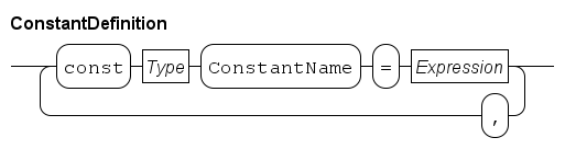
An example:
const real speed = 4.8,
      dict(string : list int) recipes = { "short" : [1,4,8],
                                          "long"  : [1,1,2,3,4,5] };
Here, a speed real value is defined, and recipes value, a dictionary of string to numbers.
The constant names can be used at every point where you can use an expression.
See the Expressions section for details about expressions.
Note that you cannot use a constant name in its own definition.
Process definitions
A process is an entity that shows behavior over time. A process definition is a template for such a process. It is defined as follows.
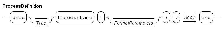
The definition starts with the keyword proc optionally followed by an exit type.
The name of the process definition, and its formal parameters concludes the header.
In the body, the behavior is described using statements.
Formal parameters are further explained in Formal parameters, statements are explained in the Statements section.
For example:
proc P():
  writeln("Hello");
  delay 15;
  writeln("Finished")
end
In the example, a process definition with the name P is defined, without parameters, that outputs a line of text when starting, and another line of text 15 time units later (and then finishes execution).
Creating and running a process is done with Sub-process statements (start or run) from another process or from a model.
If a process definition has no exit type specified, it may not use the exit statement, nor may it start other processes that have an exit type (see also Sub-process statements).
Process definitions that have an exit type may use the exit statement directly (see Exit statement for details on the statement), and it may start other processes without exit type, or with the same exit type.
Since values returned by the exit statement may get printed onto the output, you may only use exit types that are printable.
These are all the 'normal' data values, from simple booleans to lists, sets, and dictionaries of data values, but not channels, files, etc.
Model definitions
A model behaves like a process, the only difference is that a model is run as first process. It is the 'starting point' of a simulation. As such, a model can only take data values which you can write down as literal value. For example, giving it a channel or a process instance is not allowed.
Like the process, a model also has a definition. It is defined below.
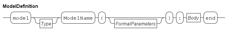
The syntax is exactly the same as process definitions explained in Process definitions, except it starts with a model keyword instead.
A model can be started directly in the simulator (see Software operation), or as part of an experiment, explained in Simulating several scenarios, and Experiment definitions.
If the model definition has no exit type, it may not use the exit statement directly, nor may it start other processes that have an exit type.
If an exit type is specified, the model may use the exit statement to end the model simulation (see Sub-process statements for details), and it may start other processes, either without exit type, or with a matching exit type.
Function definitions
In programs, computations are executed to make decisions. These computations can be long and complex. A function definition attaches a name to a computation, so it can be moved to a separate place in the file.
Another common pattern is that the same computation is needed at several places in the program. Rather than duplicating it (which creates consistency problems when updating the computation), write it in a function definition, and call it by name when needed.
The syntax of a function definition is as follows.
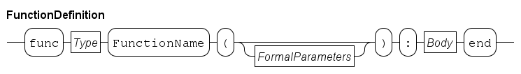
In the syntax, the only thing that changes compared with the syntax in Process definitions or Model definitions is the additional Type node that defines the type resulting from the computation.
However, since a function represents a computation (that is, calculation of an output value from input values) rather than having behavior over time, the Body part has additional restrictions.
-
A computation is performed instantly, no time passes. This means that you cannot delay or wait in a function.
-
A computation outputs a result. You cannot have a function that has no result.
-
A computation is repeatable. That means if you run the same computation again with the same input values, you get the same result every time. Also in the environment of the function, there should be no changes. This idea is known as mathematical functions.
A consequence of having mathematical functions is that you cannot interact with 'outside'. No querying of the current time, no communication, no select statement, and no use of distributions.
Technically, this would also imply no input/output, but for practical reasons this restriction has been lifted. However, as a general rule, avoid using it.
Experiment definitions
An experiment can execute one or more model simulations, collect their exit values, and combine them into a experiment result. Its syntax is shown below.
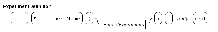
An experiment definition has some function-like restrictions, like not being able to use sub-process statements, no communication, and no use of time. On the other hand, it does not return a value, and it can start model simulations that have a non-void exit type (Void type discusses the void type).
The definition is very similar to other definitions.
It starts with an xper keyword, followed by the name of the definition.
The name can be used to start an experiment with the simulator (see Software operation for details on starting the simulator).
If formal parameters are specified with the experiment definition (see Formal parameters below), the experiment can be parameterized with values.
Like models, an experiment can only take data values which you can write down as literal value.
For example, giving it a channel or a process instance is not allowed.
The body of an experiment is just like the body of a Function definitions (no interaction with processes or time). Unlike a function, an experiment never returns a value with the Return statement.
The primary goal of an xper is to allow you to run one or more model simulations that give an exit value.
For this purpose, you can 'call' a model like a function, for example:
xper X():
    real total;
    int n;

    while n < 10:
        total = total + M();
        n = n + 1
    end

    writeln("Average is %.2f", total / 10);
end

model real M():
    dist real d = exponential(7.5);
    exit sample d;
end
The model above is very short to keep the example compact.
In practice it will be larger, start several concurrent processes, and do a lengthy simulation before it decides what the answer should be.
The experiment X makes ten calls to the model.
Each call causes the model to be run, until the model or one of its processes executes the exit statement.
At that point, the model and all its processes are killed, and the value supplied with the exit statement becomes the return value of the model call, adding it to total.
After the ten model simulations, the experiment outputs the average value of all model simulations.
Note that the called model (or one of its started processes) must end with the exit statement, it is an error when the model ends by finishing its last model statement.
Formal parameters
Definitions above often take values as parameter to allow customizing their behavior during execution. The definition of those parameters are called formal parameters. The syntax of formal parameters is shown below.
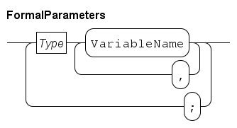
As you can see, they are just variable declarations (explained in the Local variables section), except you may not add an initial value, since their values are obtained during use of the definition.
To a definition, the formal parameters act like variables. You may use them just like other variables.
An example, where int x, y; string rel are the formal parameters of process definition P:
proc P(int x, y; string rel):
    writeln("%d %s %d", x, rel, x-y)
end

...

run P(2, -1, "is less than");
The formal parameters introduce additional variables in the process, that can be just like any other variable. Here, they are just printed to the screen. Elsewhere in the program, the definition gets used (instantiated), and a value is supplied for the additional variables. Such values are called actual parameters.
Statements
Statements express how a process or function in a system works. They define what is done and in which order. Many statements use data for their decisions, which is stored in local variables. The combined local variables and statements are called 'body' with the following syntax.
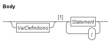
Data values available to the process are the global constants (see Constant definitions) and enumeration values (see Enumeration definitions). The formal parameters of the surrounding process definition (explained in Process definitions) or the surrounding function definition (explained in Function definitions) are added as well.
Data storage that can be modified by the process are the local variables, defined by the VarDefinitions block in the Body diagram above (variable definitions are explained below in Local variables).
The data values and the modifiable data storage is used by the statements of the Body in the path after 1.
For ease of reference they are grouped by kind of statement as shown in the Statement diagram below.
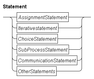
-
The
AssignmentStatementis used to assign new values to the local variables (and explained further in Assignment statement). -
The
IterativeStatementallows repeated execution of the same statements by means of theforandwhilestatements (further explained in Iterative statements). -
The
ChoiceStatementallows selection on which statement to perform next by means of theifstatement (explained in Choice statement). -
The
runandstartstatements of theSubProcessStatementgroup (explained in Sub-process statements) start new processes. -
Communication with other processes using channels is done with send, receive, and
selectstatements inCommunicationStatement(explained in Communication statements) -
Finally, the
OtherStatementsgroup contains several different statements (explained further in Other statements). The more commonly used statements in that group are thedelaystatement, thewritestatement, and thereturnstatement.
The syntax diagram of Body states that statements are separated from each other with a semicolon (;).
The compiler allows more freedom.
Semicolons may be omitted before and after a end keyword, and a semicolon may be added after the last statement.
Local variables
Local variables are introduced in a process or function using the following syntax.
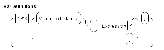
Variable definitions start with a Type node (its syntax if explained in Types), followed by a sequence of variable names where each variable may be initialized with a value by means of the = Expression path.
If no value is assigned, the variable gets the default value of the type.
Use a semicolon to terminate the sequence of new variables.
Next, another set of variables may be defined by going back to the start of the diagram, and giving another Type node, or the diagram can be ended, and the statements of the process or function can be given.
Assignment statement
An assignment statement assigns one or more values to the local variables. Its syntax is as follows.
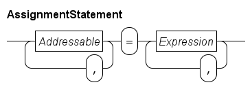
The assignment statement computes the value of every Expression at the right.
If there is one expression, its value is also the value to assign.
If there are more expressions, a tuple value is constructed, combining all values into one tuple (see Tuple expression for a discussion of tuple values).
At the left, a number of Addressable blocks define where the computed value is assigned to.
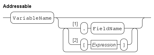
An Addressable is a variable.
If the variable has a tuple type (see Tuple type) a field of the tuple may be assigned only using Path 1.
Similarly, if the variable is a list (see List type) or a dictionary (see Dictionary type) assignment is done to one element by using Path 2.
The Expression here is evaluated before any assignment by this statement is performed.
Since selected elements may also have a type that allows selection, element selection can be repeated.
After processing the element selections at the left, it is known where values are assigned to. If there is exactly one addressable at the left, its type must match with the type of the value at the right (which may be a constructed tuple value as explained above). The value gets copied into the variable (or in its element if one is selected). If there are several addressable values at the left, the number of values must be equal to the length of the tuple from the expression(s) at the right, and each field of the right tuple must pair-wise match with the type of the addressed element at the left. In the latter case, all assignments are done at the same moment.
For a few examples, a number of variable declarations are needed:
int x, y;
real r;
list(10) int xs;
tuple(real v; int w) t;
func tuple(real v; int w) (int) f;

...  # Initialization of the variables omitted
The variable declarations introduce integer variables x and y, a real number variable r, a list of 10 integers xs, a tuple t with two fields, and a function variable f.
For reasons of clarity, initialization of the variables has been omitted. Also, expressions at the right are simple values. However, you may use all allowed expression operations explained in the next chapter (Expressions) to obtain a value to assign. The first assignments show assignment of values to variables where there is one explicit value for every assigned variable:
x = 3;
t = f(y);
x, y = 4, 5;
xs[0], t.v = x+x, r;
The first assignment statement assigns 3 to x.
The second assignment assigns the return value of the function call f(y) to tuple t.
The third assignment assigns 4 to x and 5 to y at the same time.
The fourth assignment assigns the value of x+x to the first element of the list xs, and the value of r to the v field of tuple t.
The next assignments show combining or splitting of tuples:
t = r, y;
r, x = t;
r, x = f(y);
The first assignment assigns a new value to every field of tuple t (t.v gets the value of r, while t.w gets the value of y).
This is called packing, it 'packs' the sequence of values into one tuple.
The opposite operation is demonstrated in the second assignment.
The value of each field of t is assigned to a separate variable.
The types of the variables at the left have to pair-wise match with the field types of the tuple at the right.
This assignment is called unpacking, it 'unpacks' a tuple value into its separate elements.
The third assignment does the same as the second assignment, the difference is that the value at the right is obtained from a function call.
The origin of the value is however irrelevant to the assignment statement.
To demonstrate the order of evaluation, the following assignment, under the assumption that variable x holds value 3:
x, xs[x-1] = 7, x+2;The assignment first computes all values at the right. Since there are more than one expression, they are combined into a tuple:
x, xs[x-1] = (7, 5);Next, the addressable values are calculated:
x, xs[2] = (7, 5);Finally the values are assigned, x gets a new value 7, while the third element of xs gets the value of expression x+2.
The expressions at the right as well as the expressions to select elements in lists and dictionaries are always evaluated using values from before the assignment.
It is forbidden to assign the same variable or selected element more than once:
x, x = 3, 3         # Error, assigned 'x' twice.
xs[0], xs[1] = 0, 1 # Allowed, different selected elements.
xs[0], xs[x] = 0, 1 # Allowed if x != 0.
Iterative statements
The iterative statements are shown below.
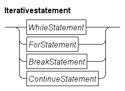
The Chi language has two statements for repeatedly executing a body (a sequence of statements), a while statement and a for statement.
The former is the generic iterative statement, the latter simplifies the common case of iterating over a collection of values.
The break and continue statements change the flow of control in the iterative statements.
While loop statement
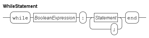
A while loop starts with the keyword while with a boolean condition.
Between the colon and the end keyword, the body of statements is given, which is executed repeatedly.
Executing an iterative while statement starts with evaluating the boolean condition.
If it does not hold, the while statement ends (and execution continues with the statement following the while statement).
If the condition holds, the statements in the body are executed from start to end (unless a break or continue statement is executed, as explained below).
After the last statement has been executed, the while statement starts again from the beginning, by evaluating the boolean condition again.
As an example, consider the following code:
int s, i;

while i < 10:
    s = s + i
    i = i + 1
end
At first, the i < 10 condition holds, and the body of the while statement (two assignment statements) is executed.
After the body has finished, i has been incremented, but is still less than 10.
The condition again holds, and the body is again executed, etc.
This process continues, until the final statement of the body increments i to 10.
The condition does not hold, and execution of the while statement ends.
For loop statement
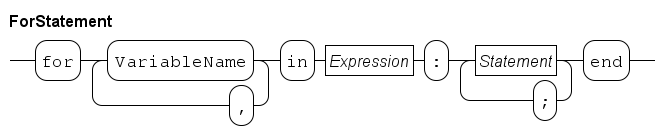
A common case for iterating is to execute some statements for every value in a collection, for example a list:
list int xs;
int x;
int i;

while i < size(xs):
    x = xs[i]
    ...
    i = i + 1
end
where the ... line represents the statements that should be executed for each value x of the list.
This is a very common case.
Chi has a special statement for it, the for statement.
It looks like:
list int xs;

for x in xs:
    ...
end
This code performs the same operation, the statements represented with ... are executed for each value x from list xs, but it is shorter and easier to write.
The advantages are mainly a reduction in the amount of code that must be written.
-
No need to create and update the temporary index variable
i. -
Variable
xis declared implicitly, no need to write a full variable declaration for it.
The behavior is slightly different in some circumstances.
-
There is no index variable
ithat can be accessed afterwards. -
When the
...statements modify the source variable (xsin the example), thewhilestatement above uses the changed value. Theforstatement continues to use the original value of the source variable.
Continuing use of the original source value can be an advantage or a disadvantage, depending on the case.
Using the new value gives more flexibility, keeping the old value makes the for statement more predictable, for example indices in the source variable stay valid.
Besides iterating over a list with for, you can also iterate over element values of a set, or over key-value tuples of a dictionary, for example:
dict(int:int) d = {1:10, 2:20};

for k, v in d:
    writeln("%s: %s", k, v);
end
When iterating over a set or a dictionary, the order of the elements is undefined.
In the above example, the first pair is either (1, 10) or (2, 20).
Break statement
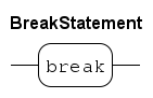
The break statement may only be used inside the body of a loop statement.
When executed, the inner-most loop statement ends immediately, and execution continues with the first statement after the inner-most loop statement.
An example:
# Get a slice of the xs list, up-to the position of value x in the list
func get_until(list int xs, int x):
    int index;

    while index < size(xs):
        if xs[index] == x:
            break
        end;
        index = index + 1
    end
    return xs[:index]
end
In the example, elements of the list xs are inspected until an element with a value equal to x is found.
At that point, the loop ends with the break statement, and the function returns a slice of the list.
Continue statement
Another common case when executing the body of an inner-most loop is that the remaining statements of the body should be skipped this time.
It can be expressed with an if statement, but a continue statement is often easier.
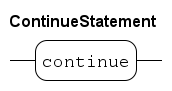
The syntax of the continue statement is just continue.
An example to demonstrate its operation:
int s;

for x in xs:
    if x mod 5 == 0:
        continue
    end
    s = s + x
end
The for statement iterates over every value in list xs.
When the value is a multiple of 5 (expressed by the condition x mod 5 == 0), the continue is executed, which skips the remaining statements of the body of the for statement, namely the s = s + x assignment.
The result is that after executing the for statement, variable s contains the sum of all values of the list that are not a multiple of 5.
Choice statement
The choice statement, also known as 'if statement', selects one alternative from a list based on the current value of a boolean expression.
The alternatives are tried in turn, until a boolean expression one an alternative yields true.
The statements of that alternative are executed, and the choice statement ends.
The choice statement also ends when all boolean expressions yield false.
The boolean expression of the else alternative always holds.
The syntax of the choice statement is as follows.
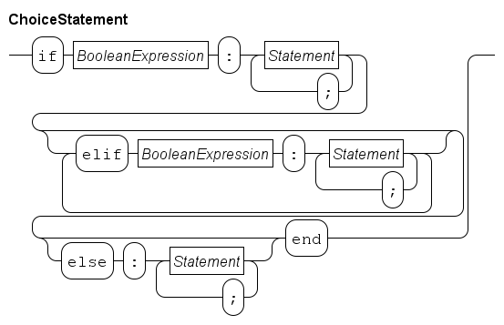
Processing starts with evaluating the BooleanExpression behind the if.
If it evaluates to true, the statements behind it are executed, and the choice statement ends.
If the boolean expression behind the if does not hold, the sequence elif alternatives is tried.
Starting from the first one, each boolean expression is evaluated.
If it holds, the statements of that alternative are performed, and the choice statement ends.
If the boolean expression does not hold, the next elif alternative is tried.
When there are no elif alternatives or when all boolean expressions of the elif alternatives do not hold, and there is an else alternative, the statements behind the else are executed and the choice statement ends.
If there is no else alternative, the choice statement ends without choosing any alternative.
An example with just one alternative:
if x == 1:
    x = 2
end
which tests for x == 1.
If it holds, x = 2 is performed, else no alternative is chosen.
An longer example with several alternatives:
if x == 1:
     y = 5
elif x == 2:
    y = 6; x = 6
else:
    y = 7
end
This choice statement first tests whether x is equal to 1.
If it is, the y = 5 statement is executed, and the choice statement finishes.
If the first test fails, the test x == 2 is computed.
If it holds, the statements y = 6; x = 6 are performed, and the choice statement ends.
If the second test also fails, the y = 7 statement is performed.
The essential points of this statement are:
-
The choice is computed now, you cannot wait for a condition to become true.
-
Each alternative is tried from the top down, until the first expression that yields true.
The second point also implies that for an alternative to be chosen, the boolean expressions of all previous alternatives have to yield false.
In the above example, while executing the y = 7 alternative, you know that x is neither 1 nor 2.
Sub-process statements
The sub-process statements deal with creating and managing of new processes. The statement may only be used in Process definitions and Model definitions.
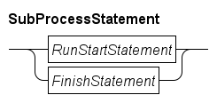
The RunStartStatement block creates new processes (see Run and start statements for details), while the FinishStatement waits for a process to end (further explanation at Finish statement).
Run and start statements
The run and start commands take a sequence of process instance as their argument.
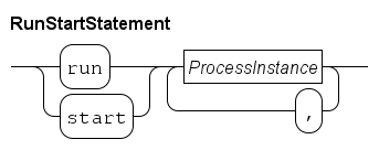
Both statements start all instances listed in the sequence.
The start statement ends directly after starting the processes, while the run statement waits until all the started instances have ended.
Using run is generally recommended for creating new processes.
A process instance has the following syntax.
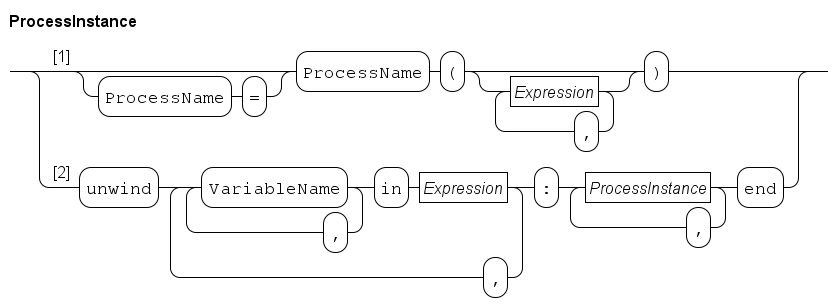
The elementary process instance is created using Path 1. It consists of a process name (which must be one of the names of the Process definitions), followed by a sequence of actual parameters for the process between parentheses. The number of actual parameters and their types must match pair-wise with the number and type of the formal parameters of the referenced process definition. Channel directions of the formal parameters must be a sub-set of the channel directions of the actual parameters.
The optional assignment of the process to a process variable (which must be of type inst, see Instance type) allows for checking whether the started process has ended, or for waiting on that condition in a select statement (explained in Select statement), or with a finish statement (explained in Finish statement).
For example:
chan c;
inst p, q;

run P(18, c), Q(19, c);
start p = P(18, c), q = Q(19, c);
First two processes are completely run, namely the instances P(18, c), and Q(19, c).
When both have ended, the start statement is executed, which starts the same processes, and assigned the P process instance to instance variable p and the Q process instance to variable q.
After starting the processes, the start ends.
Unless one of started processes has already ended, in the statement following the start, three processes are running, namely the process that executed the start statement, and the two started process instances referenced by variables p and q.
(There may be more processes of course, created either before the above statements were executed, or the P or Q process may have created more processes.)
Path 2 of the ProcessInstance diagram is used to construct many new processes by means of an unwind loop.
Each value in the Expression gets assigned to the iterator variable sequence of VariableName blocks (and this may be done several times as the syntax supports several Expression loops).
For each combination of assignments, the process instances behind the colon are created.
The end keyword denotes the end of the unwind.
Typical use of unwind is to start many similar processes, for example:
list int xs = [1, 2]

run
    unwind i in range(5),
           j in range(3),
           x in xs: P(i, j, x)
    end;
This run statement runs 5*3*2 processes: P(0, 0, 1), P(0, 0, 2), P(0, 1, 1), …, P(0, 2, 2), P(1, 0, 1), …, P(4, 2, 2).
Both the run and the start statements can always instantiate new processes that have no exit type specified.
(see Process definitions for details about exit types in process definitions).
If the definition containing the sub-process statement has an exit type, the statements can also instantiate processes with the same exit type.
This requirement ensures that all exit statements in a model simulation give exit values of the same type.
Finish statement
The finish statement allows waiting for the end of a process instance.
The statement may only be used in Process definitions and Model definitions.
Its syntax is as follows.
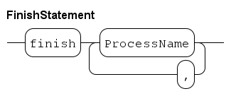
Each process variable must be of type inst (see Instance type for details).
The statement ends when all referenced process instances have ended.
For example:
chan bool c;
inst p, q;

start p = P(18, c), q = Q(19, c);
finish p, q;
During the start statement (see Run and start statements), instance variables p and q get a process instance assigned (this may also happen in different start statements).
The finish statement waits until both process instances have ended.
Communication statements
Communication with another process is the only means to forward information from one process to another processes, making it the primary means to create co-operating processes in the modeled system. The statement may only be used in Process definitions and Model definitions.
All communication is point-to-point (from one sender to one receiver) and synchronous (send and receive occur together). A communication often exchanges a message (a value), but communication without exchange of data is also possible (like waving 'hi' to someone else, the information being sent is 'I am here', but that information is already implied by the communication itself). The latter form of communication is called synchronization.
Send and receive does not specify the remote process directly, instead a channel is used (see Channel type and Channel expressions sections for more informations about channels and how to create them). Using a channel increases flexibility, the same channel can be used by several processes (allowing communication with one of them). Channels can also be created and exchanged during execution, for even more flexibility.
Setting up a communication channel between two processes is often done in the following way:
chan void sync;   # Synchronization channel
chan int  dch;    # Channel with integer number messages

run P(sync, dch), Q(sync, dch);
In a parent process, two channels are created, a synchronization channel sync, and a communication channel with data called dch.
The channel values are given to processes P and Q through their formal parameters.
The communication statements are as follows.
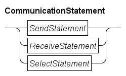
The elementary communication statements for sending and receiving at a single channel are the Send statement and the Receive statement. The Select statement is used for monitoring several channels and conditions at the same time, until at least one of them becomes available.
Send statement
The send statement send signals or data away through a channel. The statement may only be used in Process definitions and Model definitions. It has the following syntax:
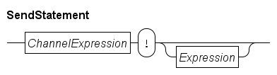
The statement takes a channel value (derived from ChannelExpression), and waits until another process can receive on the same channel.
When that happens, and the channel is a synchronization channel, a signal 'Communication has occurred' is being sent, if the channel also carries data, the Expression value is computed and sent to the other process.
For example:
proc P(chan void a, chan! int b):
    a!;
    b!21;
end
Process P takes two parameters, a synchronization channel locally called a and a outgoing channel called b carrying integer values.
In the process body, it first synchronizes over the channel stored in a, and then sends the value 21 of the channel stored in b.
Receive statement
The receive statement receives signals or data from a channel. The statement may only be used in Process definitions and Model definitions. It has the following syntax:
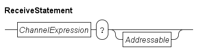
The statement takes a channel value (derived from the ChannelExpression), and waits until another process can send on the same channel.
For synchronization channels, it receives just a signal that the communication has occurred, for channels carrying data, the data value is received and stored in the variable indicated by Addressable.
For example:
proc Q(chan void a, chan int b):
    int x;

    a?;
    b?x;
    writeln("%s", x);
end
Process Q takes a synchronization channel called a and a data channel for integer values called b as parameters.
The process first waits for a synchronization over channel a, and then waits for receiving an integer value over channel b which is stored in local variable x.
Select statement
The Send statement and the Receive statement wait for communication over a single channel. In some cases, it is unknown which channel will be ready first. Additionally, there may be time-dependent internal activities that must be monitored as well. The select statement is the general purpose solution for such cases. The statement may only be used in Process definitions and Model definitions.
It has the following syntax:
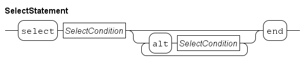
The statement has one or more SelectCondition alternatives that are all monitored.
The first alternative is prefixed with select to denote it is a the start of a select statement, the other alternatives each start with alt (which is an abbreviation of 'alternative').
The statement monitors all conditions simultaneously, waiting for at least one to become possible. At that moment, one of the conditions is selected to be executed, and the select statement ends.
The syntax of a SelectCondition is:
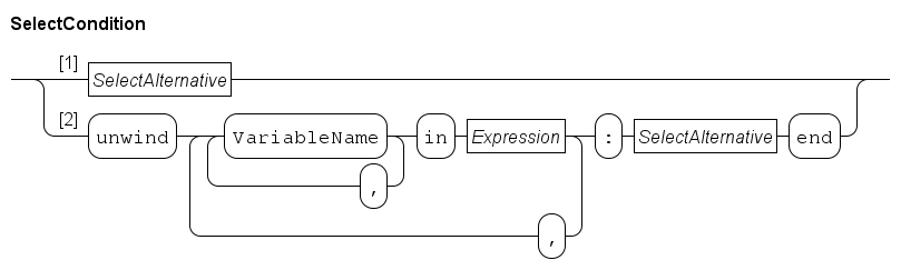
In its simplest form, a SelectCondition is a SelectAlternative (taking Path 1).
At Path 2, the condition is eventually also an SelectAlternative, but prefixed with an unwind construct, and with an additional end keyword at the end to terminate the unwind.
The unwind construct allows for a compact notation of a large number of alternatives that must be monitored. Examples are provided below.
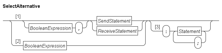
Using Path 1, a SelectAlternative can be a Send statement or a Receive statement, which may optionally have a BooleanExpression condition prefix.
Path 2 allows for a condition without a send or receive statement.
The alternative checks the condition and monitors the channel. If the condition holds and the channel has a communication partner, the alternative can be chosen by the select statement. (Of course, omitting a condition skips the check, and not specifying a send or receive statement skips monitoring of the channel.) When an alternative is chosen by the select statement, the send or receive statement are performed (if it was present). If additional statements were given in the alternative using Path 3, they are executed after the communication has occurred (if a send or receive was present).
A few examples to demonstrate use of the select statement:
timer t = timer(5.2);

select
    a?
alt
    b!7:
        writeln("7 sent")
alt
    ready(t):
        writeln("done")
end
This select waits until it can receive a signal from channel a, it can send value 7 over channel b, or until ready(t) holds (which happens 5.2 time units after starting the select, see Timers for details).
If b!7 was selected, the writeln("7 sent") is executed after the communication over channel b.
If the ready(t) alternative is chosen, the writeln("done") is executed.
A buffer can be specified with:
list int xs;
int x;

select
    a?x:
        xs = xs + [x]
alt
    not empty(xs), b!xs[0]:
        xs = xs[1:]
end
The select either receives a value through channel a, or it sends the first element of list xs over channel b if the list is not empty (the condition must hold and the channel must be able to send an item at the same time to select the second alternative).
After communication has been performed, the first alternative appends the newly received value x to the list (the received value is stored in x before the assignment is executed).
In the second alternative, the assignment statement drops the first element of the list (which just got sent away over channel b).
The unwind loop 'unwinds' alternatives, for example:
list(5) chan int cs;
int x;

select
    unwind i, c in enumerate(cs):
        c?x:
            writeln("Received %s from channel number %d", x, i)
    end
end
Here cs is a list of channels, for example list(5) chan int cs.
(See List type for details about lists.) The unwind iterates over the enumerate(cs) (see List expressions for details about enumerate), assigning the index and the channel to local i and c variables.
The SelectAlternative uses the variables to express the actions to perform (wait for a receive, and output some text saying that a value has been received).
The above is equivalent to (if list cs has length 5):
select
    cs[0]?x:
        writeln("Received %s from channel number %d", x, 0)
alt
    cs[1]?x:
        writeln("Received %s from channel number %d", x, 1)

...

alt
    cs[4]?x:
        writeln("Received %s from channel number %d", x, 4)
The unwind however works for any length of list cs.
In addition, the unwind allows for nested loops to unfold for example list list bool ds, or to send one of several values over one of several channels.
Other statements
Finally, there are a number of other useful statements.
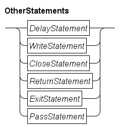
The Delay statement waits for the given amount of time units, the Write statement outputs text to the screen or a file, the Close statement closes a file, the Return statement returns a value from a function. the Exit statement ends the execution of all processes, and the Pass statement does nothing.
Delay statement
The delay statement is useful to wait some time.
The statement may only be used in Process definitions and Model definitions.
It has the following syntax:
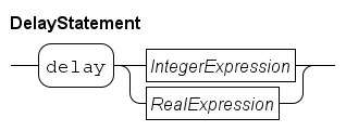
The IntegerExpression or RealExpression is evaluated, and is the amount of time that the statement waits.
The value of the expression is computed only at the start, it is not evaluated while waiting.
Changes in its value has thus no effect.
A negative value ends the statement immediately, you cannot go back in time.
Examples:
delay 1.5 # Delay for 1.5 time units.
Write statement
The write statement is used to output text to the screen or to a file. It has the following syntax:
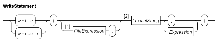
The format string at 2 is a literal string value (further explained at String expressions) which defines what gets written.
Its text is copied to the output, except for two types of patterns which are replaced before being copied.
Use of the writeln (write line) keyword causes an additional \n to be written afterwards.
The first group of pattern are the back-slash patterns.
They all start with the \ character, followed by another character that defines the character written to the output.
The back-slash patterns are listed in the table below.
| Pattern | Replaced by |
|---|---|
|
The new-line character (U+000A) |
|
The tab character (U+0009) |
|
The double-quote character (U+0022) |
|
The back-slash character (U+005C) |
The second group of patterns are the percent patterns.
Each percent pattern starts with a % character.
It is (normally) replaced by the (formatted) value of a corresponding expression listed after the format string (the first expression is used as replacement for the first percent pattern, the second expression for the second pattern, etc).
How the value is formatted depends on the format specifier, the first letter after the percent character.
Between the percent character and the format specifier may be a format definition giving control on how the value is output.
The format definition consists of five parts, each part is optional.
-
A
-character, denoting alignment of the value to the left. Cannot be combined with a0, and needs a width. -
A
+character, denoting the value with always be printed with a sign, only for formatting decimal integers, and real numbers. -
A
0character, denoting the value will be prefixed with zeros, only for integer numbers. Cannot be combined with-, and needs a width. -
A width as decimal number, denoting the minimal amount of space used for the value. The value will be padded with space (or zeros if the
0part has been specified). -
A
.and a precision as decimal number, denoting the number of digits to use for the fraction, only for real numbers.
The format definition is a single letter, the table below lists them and their function.
| Definition | Description |
|---|---|
|
Output boolean value. |
|
Output integer value as decimal number. |
|
Output integer value as hexadecimal number. |
|
Output real value as number with a fraction. |
|
Output real value in exponential notation. |
|
Output real value either as |
|
Output value as a string (works for every printable value) |
|
Output a |
Close statement
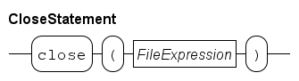
The close statement takes a value of type file as argument (see File type for details about the file type).
It closes the given file, which means that the file is no longer available for read or write.
In case data was previously written to the file, the close statement ensures that the data ends up in the file itself.
Note that a close of a file is global in the system, none of the processes can use the file any longer.
In Reading from a file and Writing to a file, use of the close statement is shown.
Return statement
The return statement may only be used in a Function definitions. It has the following syntax:
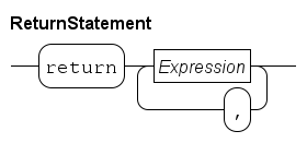
The statement starts with a return keyword, followed by one or more (comma-separated) expressions that form the value to return to the caller of the function.
The value of the expressions are calculated, and combined to a single return value.
The type of the value must match with the return type of the function.
Execution of the function statements stops (even when inside a loop or in an alternative of an if statement), and the computed value is returned to the caller of the function.
Examples:
return 4          # Return integer value 4 to the caller.

return true, 3.7  # Return value of type tuple(bool b; real r).
Exit statement
The exit statement may only be used in Process definitions and Model definitions.
It has the following syntax:
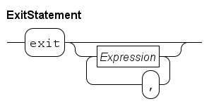
The exit statement allows for immediately stopping the current model simulation. The statement may be used in Process definitions and Model definitions. If arguments are provided, they become the exit value of the model simulation. Such values can be processed further in an Simulating several scenarios, see also Experiment definitions on how to run a model in an experiment.
The type of the combined arguments must match with the exit type of the process or model that uses the statement.
If no arguments are given, the exit type must be a void type (see also Void type).
If an experiment is running, execution continues by returning from the model instantiation call. Otherwise, the simulation as a whole is terminated.
Pass statement
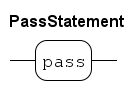
The pass statement does nothing.
Its purpose is to act as a place holder for a statement at a point where there is nothing useful to do (for example to make an empty process), or to explicitly state nothing is being done at some point:
if x == 3:
    pass
else:
    x = x + 1
end
Here, pass is used to explicitly state that nothing is done when x == 3.
Such cases are often a matter of style, usually it is possible to rewrite the code and eliminate the pass statement.
Expressions
Expressions are computations to obtain a value. The generic syntax of an expression is shown below.
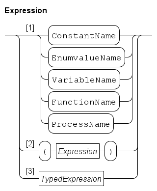
-
As shown in Path 1, a name may be used in an expression. It must refer to a value that can be used in an expression. Names are explained further at Names.
The first four entries are quite normal, function names can be used for variables with a function type (see Function type) and process names for variables with a process type (see Process type). The latter two are mainly useful as actual parameters of functions or processes.
-
Path 2 states that you can write parentheses around an expression. Its main use is to force a different order of applying the unary and binary operators (see Operator priorities). Parentheses may also be used to clarify the meaning of a complicated expression.
-
Path 3 gives access to the other parts of expressions. Typed expressions gives the details about typed expressions.
Typed expressions
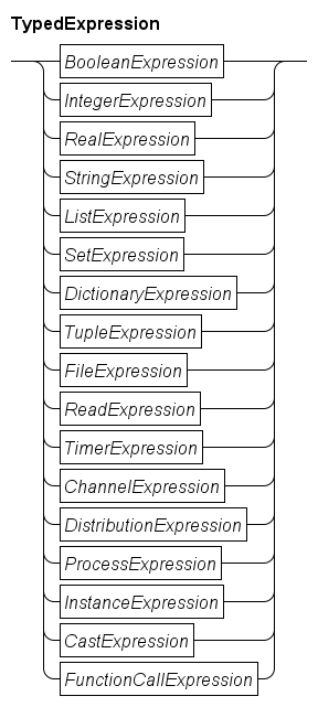
The number of operators in expressions is quite large.
Also, each node has an associated type, and the allowed operators depend heavily on the types of the sub-expressions.
To make expressions easier to access, they have been split.
If possible the (result) type is leading, but in some cases (like the ReadExpression for example) this is not feasible.
-
The expressions with a boolean type are denoted by the
BooleanExpressionblock and explained further in Boolean expressions. -
The expressions with an integer type are denoted by the
IntegerExpressionblock and explained further in Integer expressions. -
The expressions with a real number type are denoted by the
RealExpressionblock and explained further in Real number expressions. -
The expressions with a string type are denoted by the
StringExpressionblock and explained further in String expressions. -
The expressions with a list type are denoted by the
ListExpressionblock and explained further in String expressions. -
The expressions with a set type are denoted by the
SetExpressionblock and explained further in Set expressions. -
The expressions with a dictionary type are denoted by the
DictionaryExpressionblock and explained further in Dictionary expressions. -
The expressions with a tuple type are denoted by the
TupleExpressionblock and explained further in Tuple expression. -
The expressions with a file handle type are denoted by the
FileExpressionblock and explained further in File handle expressions. -
The function to read values from an external source is shown in the
ReadExpressionblock, and further discussed in Read expression. -
The expressions with a timer type are denoted by the
TimerExpressionblock and explained further in Timer expressions. -
The expressions with a channel type are denoted by the
ChannelExpressionblock and explained further in Channel expressions. -
The expressions with a distribution type are denoted by the
DistributionExpressionblock and explained further in Distribution expressions. -
The expressions with a process type are denoted by the
ProcessExpressionblock and explained further in Process expressions. -
The expressions with an instance type are denoted by the
InstanceExpressionblock and explained further in Instance expressions. -
The expressions that convert one type to another are denoted by the
CastExpressionblock, and explained further in Cast expressions. -
The expressions that perform a function call are denoted by the
FunctionCallExpressionblock, and explained further in Function call expressions.
Enumeration value
Enumeration values may be used as literal value in an expression.
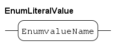
See Enumeration definitions for a discussion about enumeration definitions and enumeration values.
There are two binary operators for enumeration values.
| Expression | Type lhs | Type rhs | Type result | Explanation |
|---|---|---|---|---|
lhs |
E |
E |
bool |
Test for equality |
lhs |
E |
E |
bool |
Test for inequality |
Two enumeration values from the same enumeration definition E can be compared against each other for equality (or in-equality). Example:
enum FlagColours  = {red, white, blue};

...

bool same = (red == white);
Boolean expressions
The literal values for the boolean data type are as follows.
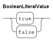
The values true and false are also the only available values of the boolean data type.
The not operation is the only boolean unary operator.
| Expression | Type op | Type result | Explanation |
|---|---|---|---|
|
bool |
bool |
op value is inverted. |
The and, the or, and the equality tests are available for boolean values.
| Expression | Type lhs | Type rhs | Type result | Explanation |
|---|---|---|---|---|
lhs |
bool |
bool |
bool |
Both operands hold |
lhs |
bool |
bool |
bool |
At least one operand holds |
lhs |
bool |
bool |
bool |
Test for equality |
lhs |
bool |
bool |
bool |
Test for inequality |
Integer expressions
The syntax of an integer literal number is (at character level) as follows.
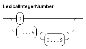
| This diagram works at lexical level (at the level of single characters), white space or comments are not allowed between elements in this diagram. |
An integer number is either 0, or a sequence of decimal digits, starting with a non-zero digit.
There are two unary operators on integer numbers.
| Expression | Type op | Type result | Explanation |
|---|---|---|---|
|
int |
int |
op value is negated. |
|
int |
int |
op value is copied. |
With the unary - operation, the sign of the operand gets toggled.
The + unary operation simply copies its argument.
There are many binary operations for integer numbers, see the table below.
| Expression | Type lhs | Type rhs | Type result | Explanation |
|---|---|---|---|---|
lhs |
int |
int |
int |
Integer addition |
lhs |
int |
int |
int |
Integer subtraction |
lhs |
int |
int |
int |
Integer multiplication |
lhs |
int |
int |
real |
Real division |
lhs |
int |
int |
int |
Integer divide operation |
lhs |
int |
int |
int |
Modulo operation |
lhs |
int |
int |
real |
Power operation |
lhs |
int |
int |
bool |
Test for less than |
lhs |
int |
int |
bool |
Test for less or equal |
lhs |
int |
int |
bool |
Test for equality |
lhs |
int |
int |
bool |
Test for inequality |
lhs |
int |
int |
bool |
Test for bigger or equal |
lhs |
int |
int |
bool |
Test for bigger than |
The divide operator / and the power operator ^ always gives a real result, integer division is performed with div.
The operation always rounds down, that is a div b == floor(a / b) for all integer values a and b.
The mod operation returns the remainder from the div, that is a mod b == a - b * (a div b).
The table below gives examples.
For clarity, the sign of the numbers is explicitly added everywhere.
| Example | Result | Explanation |
|---|---|---|
|
+1 |
|
|
+3 |
|
|
-2 |
|
|
-1 |
|
|
-2 |
|
|
+1 |
|
|
+1 |
|
|
-3 |
|
The Chi simulator uses 32 bit integer variables, which means that only values from -2,147,483,647 to 2,147,483,647 (with an inclusive upper bound) can be used. Using a value outside the valid range will yield invalid results. Sometimes such values are detected and reported.
| The technical minimum value for integers is -2,147,483,648, but this number cannot be entered as literal value due to parser limitations. |
Real number expressions
Real numbers are an important means to express values in the contiguous domain.
The type of a real number expression is a real type, see Real type for more information about the type.
The syntax of real number values is as follows.
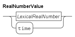
There are two ways to construct real numbers, by writing a literal real number, or by using time which returns the current time in the model.
The syntax of a literal real number (at character level) is as follows.
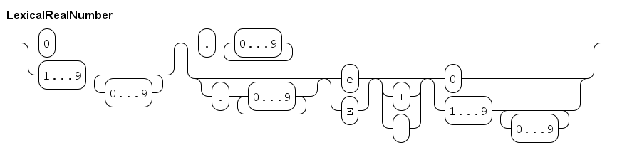
| This diagram works at lexical level (at the level of single characters), white space or comments are not allowed between elements in this diagram. |
A literal real number starts with one or more digits, and then either a dot or an exponent. In the former case, an exponent is allowed as well. Examples:
3.14
0.314e1
314E-2
A real number always has either a dot character, or an exponent notation in the number.
Many of the integer operations can also be performed on real numbers. The unary operators are the same, except for the type of the argument.
| Expression | Type op | Type result | Explanation |
|---|---|---|---|
|
real |
real |
op value is negated. |
|
real |
real |
op value is copied. |
With the unary - operation, the sign of the operand gets toggled.
The + unary operation simply copies its argument.
The binary operators on real numbers is almost the same as the binary operators on integer numbers.
Only the div and mod operations are not here.
| Expression | Type lhs | Type rhs | Type result | Explanation |
|---|---|---|---|---|
lhs |
int,real |
int,real |
real |
Addition |
lhs |
int,real |
int,real |
real |
Subtraction |
lhs |
int,real |
int,real |
real |
Multiplication |
lhs |
int,real |
int,real |
real |
Real division |
lhs |
int,real |
int,real |
real |
Power operation |
lhs |
int,real |
int,real |
bool |
Test for less than |
lhs |
int,real |
int,real |
bool |
Test for less or equal |
lhs |
int,real |
int,real |
bool |
Test for equality |
lhs |
int,real |
int,real |
bool |
Test for inequality |
lhs |
int,real |
int,real |
bool |
Test for bigger or equal |
lhs |
int,real |
int,real |
bool |
Test for bigger than |
With these operations, one of the operands has to be a real number value, while the other operand can be either an integer value or a real number value.
The standard library functions for real numbers contain a lot of math functions. They can be found in Real number functions.
The Chi simulator uses 64-bit IEEE 754 floating point numbers to represent real number values. Using a value outside the valid range of this format will yield invalid results. Sometimes such values are detected and reported.
String expressions
Strings are sequences of characters. Their most frequent use is to construct text to output to the screen. A string literal is defined as follows.
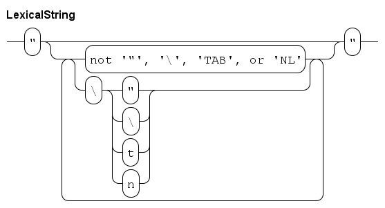
| This diagram works at lexical level (at the level of single characters), white space or comments are not allowed between elements in this diagram. |
A string literal starts with a quote character ", and ends with another quote character.
In between, you may have a sequence of characters.
Most characters can be written literally (eg write a a to get an 'a' in the string).
The exceptions are a backslash \, a quote ", a TAB, and a NL (newline) character.
For those characters, write a backslash, followed by \, ", t, or n respectively.
(A TAB character moves the cursor to the next multiple of 8 positions at a line, a NL moves the cursor to the start of the next line.)
Strings have the following binary expressions.
| Expression | Type lhs | Type rhs | Type result | Explanation |
|---|---|---|---|---|
lhs |
string |
string |
string |
Concatenation |
lhs |
string |
int |
string |
Element access |
lhs |
string |
int, int |
string |
Slicing with step |
lhs |
string |
int, int, int |
string |
Slicing |
lhs |
string |
string |
bool |
Test for less than |
lhs |
string |
string |
bool |
Test for less or equal |
lhs |
string |
string |
bool |
Test for equality |
lhs |
string |
string |
bool |
Test for inequality |
lhs |
string |
string |
bool |
Test for bigger or equal |
lhs |
string |
string |
bool |
Test for bigger than |
The concatenation operator joins two strings ("a" + "bc" gives "abc").
The element access and slicing operators use numeric indices to denote a character in the string.
First character has index value 0, second character has index 1, and so on.
Negative indices count from the back of the string, for example index value -1 points to the last character of a string.
Unlike lists, both the element access and the slicing operators return a string.
The former constructs a string with only the indicated character, while the latter constructs a sub-string where the first character is at index low, the second character at index low + step, and so on, until index value high is reached or crossed.
That final character is not included in the result (that it, the high boundary is excluded from the result).
If low is omitted, it is 0, if high is omitted, it is the length of the string (size( lhs )).
If step is omitted, it is 1.
A few examples:
string s = "abcdef";

s[4]        # results in "e"
s[2:4]      # results in "cd"
s[1::2]     # results in "bdf"
s[-1:0:-2]  # results in "fdb"
s[-1:-7:-1] # results in "fedcba"
s[:4]       # results in "abcd"
s[-1:]      # results in "f" (from the last character to the end)
In the comparison operations, strings use lexicographical order.
There are also a few standard library functions on strings, see String functions for details.
Note that length of the string is not the same as the number of characters needed for writing the string literal, as shown in the following example.
size("a")  # results in 1, string is 1 character long (namely 'a').
size("\n") # results in 1, string contains one NL character.
List expressions
Lists are very versatile data structures, the Chi language has a large number of operations and functions for them.
The most elementary list expression is a literal list. It has the following syntax.
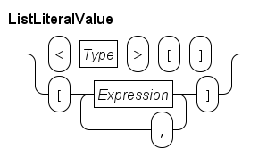
The first line shows the syntax of an empty list.
The Type block denotes the element type of the list, for example <int>[] is an empty list of integer values.
The second line shows how to write a non-empty literal list value. It is a comma-separated sequence of expressions surrounded by square brackets. The type of all expressions must be the same, and this is also the element type of the list.
Some examples:
list int xs;
list int ys = <int>[];
list int zs = [1, 4, 28];
Variable ys is assigned an empty list with integer element type.
Since an empty list is the default value of a variable, xs has the same value.
Variable zs is initialized with a list holding three elements.
Two list values are equal when they have the same number of element values, and each value is pair-wise equal.
Lists have no unary operators, the binary operators of lists are shown below.
| Expression | Type lhs | Type rhs | Type result | Explanation |
|---|---|---|---|---|
lhs |
list T |
int |
T |
Element access |
lhs |
list T |
int, int |
list T |
Slicing with step |
lhs |
list T |
int, int, int |
list T |
Slicing |
lhs |
list T |
list T |
list T |
Concatenation |
lhs |
list T |
list T |
list T |
List subtraction |
lhs |
list T |
list T |
bool |
Test for equality |
lhs |
list T |
list T |
bool |
Test for inequality |
lhs |
T |
list T |
bool |
Element test |
The element access operator 'lhs [ rhs ] ' indexes with zero-based positions, for example xs[0] retrieves the first element value, xs[1] retrieves the second value, etc.
Negative indices count from the back of the list, xs[-1] retrieves the last element of the list (that is, xs[size(xs)-1]), xs[-2] gets the second to last element, ect.
It is not allowed to index positions that do not exist.
Examples:
list int xs = [4, 7, 18];
int x;

x = xs[0];  # assigns 4
x = xs[2];  # assigns 18
x = xs[-1]; # assigns 18
x = xs[-2]; # assigns 7

xs[2]  # ERROR, OUT OF BOUNDS
xs[-4] # ERROR, OUT OF BOUNDS
The slicing operator 'lhs [ low : high ] ' extracts (sub-)lists from the lhs source.
The low and high index expressions may be omitted (and default to 0 respectively size( lhs ) in that case).
As with element access, negative indices count from the back of the list.
The result is the list of values starting at index low, and up to but not including the index high.
If the low value is higher or equal to high, the resulting list is empty.
For example:
list int xs = [4, 7, 18];
list int ys;

ys = xs[0:2];  # assigns [4, 7]
ys = xs[:2];   # == xs[0:2]
ys = xs[1:];   # == xs[1:3], assigns [7, 18]
ys = xs[:];    # == xs[0:3] == xs

ys = xs[1:2];  # assigns [7] (note, it is a list!)
ys = xs[0:0];  # assigns <int>[]
ys = xs[2:1];  # assigns <int>[], lower bound too high
ys = xs[0:-1]; # == xs[0:2]
The slicing operator with the step expression (that is, the expression with the form 'lhs [ low : high : step ] ') can also skip elements (with step values other than 1) and traverse lists from back to front (with negative step values).
Omitting the step expression or using 0 as its value, uses the step value 1.
This extended form does not count from the back of the list for negative indices, since the high value may need to be negative with a negative step size.
The first element of the result is at 'lhs [low ]'. The second element is at 'lhs [low + step ]', the third element at 'lhs [low + 2 * step ]' and so on. For a positive step value, the index of the last element is the highest value less than high, for a negative step value, the last element is the smallest index bigger than high (that is, boundary high is excluded from the result). The (sub-)list is empty when the first value ('lhs [ low ]') already violates the conditions of the high boundary.
Examples:
list int xs = [4, 7, 18];
list int ys;

ys = xs[::2];  # == xs[0:3:2], assigns [4, 18]
ys = xs[::-1]; # == xs[2:-1:-1], assigns [18, 7, 4]
With the latter example, note that the -1 end value in xs[2:-1:-1] really means index -1, it is not rewritten!
The concatenation operator + 'glues' two lists together by constructing a new list, copying the value of the lhs list, and appending the values of the rhs:
[1, 2] + [3, 4] == [1, 2, 3, 4]
<int>[] + [1]   == [1]
[5] + <int>[]   == [5]
The subtraction operator - subtracts two lists.
It copies the lhs list, and each element in the rhs list is searched in the copy, and the left-most equal value is deleted.
Searched values that do not exist are silently ignored.
The result of the operation has the same type as the lhs list.
Some examples:
[1, 2, 4, 2] - [4]        # results in [1, 2, 2], 4 is removed.
[1, 2, 4, 2] - [6]        # results in [1, 2, 4 2], 6 does not exist.
[1, 2, 4, 2] - [1, 4]     # results in [2, 2], 1 and 4 are removed.
[1, 2, 4, 2] - [2]        # results in [1, 4, 2], first 2 is removed.
[1, 2, 4, 2] - [2, 2]     # results in [1, 4].
[1, 2, 4, 2] - [2, 2, 2]  # results in [1, 4], no match for the 3rd '2'.
The element test operator in tests whether the value lhs exists in list rhs.
This operation is expensive to compute, if you need this operation frequently, consider using a set instead.
Some examples of the element test operation:
1 in [1, 2, 3]          == true
4 in [1, 2, 3]          == false  # there is no 4 in [1, 2, 3]
[1] in [[2], [1]]       == true
[2, 1] in [[1, 2]]      == false  # [2, 1] != [1, 2]
<int>[] in <list int>[] == false  # empty list contains no values.
There are also standard library functions for lists, see List functions for details.
Set expressions
Literal sets are written as follows.

The first line shows the syntax of an empty set.
The Type block denotes the element type of the set, for example <int>{} is an empty set of integer values.
The second line shows how to write a non-empty literal set value. It is a comma-separated sequence of expressions surrounded by curly brackets. The type of all expressions must be the same, and this is also the element type of the set. The order of the values in the literal is not relevant, and duplicate values are silently discarded. For example:
set real xr = {1.0, 2.5, -31.28, 1.0}assigns the set {-31.28, 1.0, 2.5} (any permutation of the values is allowed).
By convention, elements are written in increasing order in this document.
Two set values are equal when they have the same number of element values contained, and each value of one set is also in the other set. The order of the elements in a set is not relevant, any permutation is equivalent.
Like lists, sets have no unary operators. They do have binary operators though. The operators are as follows.
| Expression | Type lhs | Type rhs | Type result | Explanation |
|---|---|---|---|---|
lhs |
set T |
set T |
set T |
Set union |
lhs |
set T |
set T |
set T |
Set difference |
lhs |
set T |
set T |
set T |
Set intersection |
lhs |
set T |
set T |
bool |
Test for equality |
lhs |
set T |
set T |
bool |
Test for inequality |
lhs |
T |
set T |
bool |
Element test |
lhs |
set T |
set T |
bool |
Sub-set test |
The union of two sets means that the lhs elements and the rhs elements are merged into one set (and duplicates are silently discarded). Set difference makes a copy of the lhs set, and removes all elements that are also in the rhs operand. The result of the operation has the same type as the lhs set. Set intersection works the other way around, its result is a set with elements that exist both in lhs and in rhs. Some examples:
set int xr = {1, 3, 7};
set int yr;

yr = xr + {1, 2};  # assigns {1, 2, 3, 7}
yr = xs - {1, 2};  # assigns {3, 7}
yr = xs * {1, 2};  # assigns {1}
The element test of sets tests whether the value lhs is an element in the set rhs.
This operation is very fast.
The sub-set test does the same for every element value in the lhs operand.
It returns true is every value of the left set is also in the right set.
A few examples:
1 in {1, 3, 7}  == true
9 in {1, 3, 7}  == false

{1} sub {1, 3, 7}       == true
{9} sub {1, 3, 7}       == false
{1, 9} sub {1, 3, 7}    == false # All elements must be present.
{1, 3, 7} sub {1, 3, 7} == true # All sets are a sub-set of themselves.
There are also standard library functions for sets, see Set functions for details.
Dictionary expressions
Literal dictionaries are written using the syntax shown below.
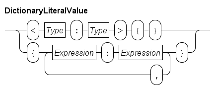
An empty dictionary needs the key and value type prefix, for example <string:int>{} is an empty dictionary with strings as key, and integer numbers as value.
Literal values of such a dictionary are:
dict(string, int) d;  # Initialized with the empty dictionary.

d = {"one": 1, "twenty-three": 23};
The key-value pairs can be put in any order. Also, the key value must be unique. Two dictionaries are equal when they have the same number of keys, each key in one dictionary is also in the other dictionary, and the value associated with each key also match pair-wise.
The binary operators of dictionaries are as follows.
| Expression | Type lhs | Type rhs | Type result | Explanation |
|---|---|---|---|---|
lhs |
dict(K:V) |
K |
V |
Element access |
lhs |
dict(K:V) |
dict(K:V) |
dict(K:V) |
Update |
lhs |
dict(K:V) |
dict(K:V) |
dict(K:V) |
Subtraction |
lhs |
dict(K:V) |
list K |
dict(K:V) |
Subtraction |
lhs |
dict(K:V) |
set K |
dict(K:V) |
Subtraction |
lhs |
dict(K:V) |
dict(K:V) |
bool |
Test for equality |
lhs |
dict(K:V) |
dict(K:V) |
bool |
Test for inequality |
lhs |
K |
dict(K:V) |
bool |
Element test |
lhs |
dict(K:V) |
dict(K:V) |
bool |
Sub-set test |
The element access operator accesses the value of a key. Querying the value of a non-existing key value is not allowed, however when used at the left side of an assignment, it acts as an adding operation. A few examples:
dict(int:bool) d = {1:true, 2:false};
bool b;

b = d[1];     # assigns 'true' (the value of key 1).
d[1] = false; # updates the value of key '1' to 'false'.
d[8] = true;  # adds pair 8:true to the dictionary.
The + operation on dictionaries is an update operation.
It copies the lhs dictionary, and assigns each key-value pair of the rhs dictionary to the copy, overwriting values copied from the lhs.
For example:
dict(int:bool) d = {1:true, 2:false};

d + {1:false}   # result is {1:false, 2:false}
d + {3:false}   # result is {1:true, 2:false, 3:false}
The subtraction operator only takes keys into consideration, that is, it makes a copy of the lhs dictionary, and removes key-value pairs where the key is also in the rhs argument (for subtraction of lists and sets, the elements are used, instead of the keys):
dict(int:bool) d = {1:true, 2:false};

d - {1:false}   # results in {2:false}, value of '1' is not relevant
d - [1]         # results in {2:false}
d - {1}         # results in {2:false}
As with list subtraction and set difference, the type of the result is the same as the type of the lhs dictionary.
The element test tests for presence of a key value, and the sub-set operation tests whether all keys of the lhs value are also in the rhs value. Examples:
dict(int:bool) d = {1:true, 2:false};
bool b;

b = 2 in d;  # assigns 'true', 2 is a key in d.
b = 5 in d;  # assigns 'false', 5 is not a key in d.

{1:false} sub d # results in 'true', all keys are in d.
There are also standard library functions for dictionaries, see Dictionary functions for details.
Tuple expression
A tuple expression is a value of a tuple type (explained in Tuple type). A tuple expression literal value is written as shown below.
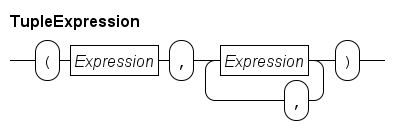
A literal tuple is a comma separated sequence of expressions of length two or longer, surrounded by a pair of parentheses. The number of expressions and the type of each expression decide the tuple type. For example:
type tup = tuple(bool b; real r);

tup t = (true, 3.48);
The type named tup is a tuple type with a boolean field and a real field.
The expression (true, 3.48) constructs the same tuple type, thus it can be assigned to variable t.
Names of the fields are not relevant in this matching, for example variable declaration (and initialization) tuple(bool z; real w) u = t is allowed, since the types of the fields match in a pair-wise manner.
A field of a tuple can be accessed both for read and for assignment by the name of the field:
bool c;

c = t.b;     # Read the 'b' field.
t.b = false; # Assign a new value to the 'b' field.
In the latter case, only the assigned field changes, all other fields keep the same value.
Tuples can also be packed and unpacked. Packing is assignment to all fields, while unpacking is reading of all fields into separate variables:
real q;

t = false, 3.8; # Packing of values into a tuple.

c, q = t;       # Unpacking into separate variables.
Packing is very closely related to literal tuples above. The difference is that packing can be done only like above in an assignment to a tuple value, while a literal tuple works everywhere.
Unpacking is very useful when the right side (t in the example) is more complex, for example, the return value of a function call, as in c, q = f();.
In such cases you don’t need to construct an intermediate tuple variable.
Packing and unpacking is also used in multi-assignment statements:
a, b = 3, 4;   # Assign 3 to 'a', and 4 to 'b'.

a, b = b, a;   # Swap values of 'a' and 'b'.
The latter works due to the intermediate tuple that is created as part in the assignment.
File handle expressions
Variables of type file are created using a variable declaration with a file type, see File type for details about the type.
You cannot write a literal value for a file type (nor can you read or write values of this type), file values are created by means of the open function in the standard library, see File functions.
You can test whether two files are the same with the binary == and != operators.
| Expression | Type lhs | Type rhs | Type result | Explanation |
|---|---|---|---|---|
lhs |
file |
file |
bool |
Test for equality |
lhs |
file |
file |
bool |
Test for inequality |
Values of type file are used for writing output to a file using the Write statement, or for reading values from a file using the read function explained in Read expression.
After use, a file should be closed with a close statement explained at Close statement.
Read expression
The read expression reads a value of a given type from the keyboard or from a file. It has two forms:
Tread(T)-
Read a value of type
Tfrom the keyboard. Tread(file f, T)-
Read a value of type
Tfrom the file opened for reading by filef(see theopenfunction in File functions for details about opening files).
You can read values from types that contain data used for calculation, that is values of types bool, int, real, string, list T, set T, and dict(K:V).
Types T, K, and V must also be readable types of data (that is, get chosen from the above list of types).
Reading a value takes a text (with the same syntax as Chi literal values of the same type), and converts it into a value that can be manipulated in the Chi model.
Values read from the text have to be constant, for example the input time cannot be interpreted as real number with the same value as the current simulation time.
Timer expressions
Timers are clocks that count down to 0.
They are used to track the amount of time you still have to wait.
Timers can be stored in data of type timer (see Timer type for details of the type).
The standard library function ready exists to test whether a timer has expired.
See Timer functions for details.
Channel expressions
Channels are used to connect processes with each other. See the Channel type for details.
Usually, channels are created by variable declarations, as in:
chan void s;
chan int c, d;
This creates three channels, one synchronization channel s, and two channels (c, and d) communicating integers.
There is also a channel function to make new channels:
chan Tchannel(T)-
Construct a new channel communicating data type
T. WhenTisvoid, a synchronization channel is created instead.
The only binary expressions on channels are equality comparison operations.
| Expression | Type lhs | Type rhs | Type result | Explanation |
|---|---|---|---|---|
lhs |
chan T |
chan T |
bool |
Test for equality |
lhs |
chan T |
chan T |
bool |
Test for inequality |
where T can be either a normal type, or void.
There has to be an overlap between the channel directions (that is, you cannot compare a receive-only channel with a send-only channel).
Distribution expressions
A distribution represents a stochastic distribution for drawing random numbers. It use a pseudo-random number generator. See Modeling stochastic behavior for a discussion how random numbers are used.
Variables of type distribution (see Distribution type) are initialized by using a distribution function from the standard library, see Distributions for an overview.
There is only one operator for variables with a distribution type, as shown below.
| Expression | Type op | Type result | Explanation |
|---|---|---|---|
|
dist bool |
bool |
Sample op distribution |
|
dist int |
int |
Sample op distribution |
|
dist real |
real |
Sample op distribution |
The sample operator draws a random number from a distribution.
For example rolling a dice:
model Dice():
    dist int d = uniform(1, 7);

    # Roll the dice 5 times
    for i in range(5):
        writeln("Rolled %d", sample d);
    end
end
Process expressions
A process expression refers to a process definition.
It can be used to parameterize the process that is being instantiated, by passing such a value to a run or start statement.
(See Run and start statements for details on how to create a new process.)
An example:
proc A(int x):
    writeln("A(%d)", x);
end

proc B(int x):
    writeln("B(%d)", x);
end

proc P(proc (int) ab):
    run ab(3);
end

model M():
    run P(A); # Pass 'proc A' into P.
end
Formal parameter ab of process P is a process variable that refers to a process taking an integer parameter.
The given process definition is instantiated.
Since in the model definition, A is given to process P, the output of the above model is A(3).
Instance expressions
Process instances represent running processes in the model. Their use is to store a reference to such a running process, to allow testing for finishing.
An instance variable is assigned during a start statement.
(See Run and start statements for details on how to start a new process.)
The instance variable is used to test for termination of the instantiated process, or to wait for it:
proc Wait():
    delay 4.52;
end

model M():
    inst w;

    start w = Wait();

    delay 1.2;
    writeln("is Wait finished? %b", finished(w));

    # Wait until the process has finished.
    finish w;
end
Wait is a process that waits a while before terminating.
In the start statement, instance variable w is set up to refer to instantiated process Wait.
After assignment, you can use the variable for testing whether the process has terminated.
In the example, the test result is written to the screen, but this could also be used as a guard in a select statement (See Select statement for details).
The other thing that you can do is to wait for termination of the process by means of the finish statement, see also Finish statement.
Matrix expression
The syntax of a matrix literal value is as follows.
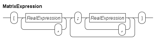
The literal starts with a [ symbol, and ends with a ] symbol.
In between it has at least two comma-separated lists of real number values, separated with a ; symbol.
Each comma-separated list of real number values is a row of the matrix. The number of columns of each row is the same at each row, which means the number of real number values must be the same with each list. As an example:
matrix(2, 3) m = [1.0, 2.0, 3.0;
                  4.0, 5.0, 6.0]
m is a matrix with two rows and three columns.
A comma separates two columns from each other, a semicolon separates two rows.
The syntax demands at least one semicolon in a literal matrix value, which means you cannot write a matrix literal with a single row directly. Instead, write a cast expression that converts a list of real numbers to a matrix with a single row. See Cast expressions for an explanation of cast expressions.
Cast expressions
A cast expression converts a value from one type to another. The syntax of a cast expression is as follows.
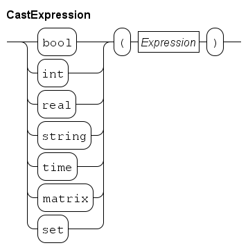
You write the result type, followed by an expression between parentheses. The value of the expression is converted to the given type. For example:
real v = 3.81;
timer t;

t = timer(v);  # Convert from real to timer (third entry in the table)
The conversion from a list to a matrix (the first entry in the table) is a special case in the sense that you also need to specify the size of the resulting matrix, as in:
list real xs = [1, 2, 3];

writeln("matrix with one row and three columns: %s", matrix(1, 3, xs));
The expected number of rows and columns given in the first two arguments must be constant. When the conversion is performed, the length of the given list must be the same as the number of columns stated in the second argument.
The number of available conversions is quite limited, below is a table that lists them.
| Value type | Result type | Remarks |
|---|---|---|
list |
matrix |
Conversion of a list to a matrix with one row |
list |
set |
Construct a set from a list |
real |
timer |
Setting up a timer |
timer |
real |
Reading the current value of a timer |
string |
bool |
Parsing a boolean value from a string |
string |
int |
Parsing an integer number from a string |
string |
real |
Parsing a real number from a string |
bool |
string |
Converting a boolean to a string representation |
int |
string |
Converting an integer to a string representation |
real |
string |
Converting a real number to a string representation |
int |
real |
Widening an integer number to a real number |
The first entry exists for creating matrices with one row (which you cannot write syntactically). The second entry constructs a set from a list of values. The element type of the list and the resulting set are the same.
The pair of conversions between timer type and real number type is for setting and reading timers, see Timers for their use.
The conversions from string to boolean or numeric allows parsing of a string. The other way around is also possible, although this is usually done as part of a write statement (see Write statement for details).
The final entry is for widening an integer to a real number. The other way around (from a real number to an integer number) does not exist as cast, but there are stdlib functions ceil, floor, and round available instead (explained in Real number functions).
Function call expressions
A function call starts a function to compute its result value from the input parameters. The syntax is as follows.
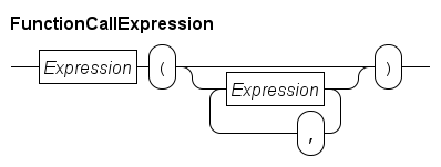
The Expression before the open parenthesis represents the function to call.
Often this is a simple name like size (the name of one of the standard library functions), but you can have more complicated expressions.
The sequence of expressions inside the parentheses denote the values of the input parameters of the functions. Their type has to match with the type stated in the formal parameter at the corresponding position.
The result of the function call is a value with the same type as stated in the return type of the function definition.
Operator priorities
Operator priorities aim to reduce the number of parentheses needed in expressions.
They do this by make choices in the order of applying operators on their arguments.
For example, 1 + 2 * 3 can be interpreted as (1 + 2) * 3 (if the addition operation is applied first), or as 1 + (2 * 3) (if the multiplication operation is performed first).
In the following table, the order of applying operators in the Chi language is defined.
| Priority | Operators |
|---|---|
1 |
(unary) |
2 |
unary |
3 |
|
4 |
|
5 |
|
6 |
|
7 |
(unary) |
8 |
|
9 |
|
Operators with a smaller priority number get applied before operators with a higher priority number. Operators with the same priority get applied from left to right.
Standard library functions
The Chi language has many general purpose functions available. They are organized by type and kind of use.
Integer functions
The following standard library functions on integers exist:
-
intabs(int val)Return the absolute value of
val. -
intsign(int val)Return
-1if val less than zero,1if val more than zero, and0otherwise. -
intmax(int a, b, ...)Return the biggest value of the parameters.
-
intmin(int a, b, ...)Return the smallest value of the parameters.
Real number functions
The following standard library functions on real numbers exist:
-
realabs(real val)Return the absolute value of
val. -
intsign(real val)Return
-1if val less than zero,1if val more than zero, and0otherwise. -
realmax(real a, b, ...)Return the biggest value of the parameters. Integer parameters are silently promoted to real.
-
realmin(real a, b, ...)Return the smallest value of the parameters. Integer parameters are silently promoted to real.
Conversion from real number to integer can be performed in three different ways.
-
intceil(real val)Return smallest integer bigger or equal to
val. -
intfloor(real val)Return biggest integer less or equal to
val. -
intround(real val)Round to nearest integer value (up if distance is
0.5).
The following power and logarithmic functions exist.
-
realsqrt(real val)Return the square root of
val(argument must be non-negative). -
realcbrt(real val)Return the cube root of
val(val^(1/3)). -
realexp(real x)Compute
e^x. -
realln(real x)Compute the natural logarithm of
x. -
reallog(real x)Compute the base-10 logarithm of
x.
Finally, there are trigonometric functions available.
-
realcos(real a)Cosine function of angle
a(in radians). -
realsin(real angle)Sine function of angle
a(in radians). -
realtan(real angle)Tangent function of angle
a(in radians). -
realacos(real val)Arc cosine function of value
val. -
realasin(real val)Arc sine function of value
val. -
realatan(real val)Arc tangent function of value
val. -
realcosh(real val)Hyperbolic cosine function of value
val. -
realsinh(real val)Hyperbolic sine function of value
val. -
realtanh(real val)Hyperbolic tangent function of value
val. -
realacosh(real val)Inverse hyperbolic cosine function of value
val. -
realasinh(real val)Inverse hyperbolic sine function of value
val. -
realatanh(real val)Inverse hyperbolic tangent function of value
val.
String functions
The following string functions exist in the standard library.
-
intsize(string s)Get the number of characters in string
s. -
stringmax(string a, b, ...)Return the biggest string of the parameters.
-
stringmin(string a, b, ...)Return the smallest string of the parameters.
List functions
Getting an element out of list can be done in two ways.
-
tuple(T value, list T ys)pop(list T xs)Get the first element of non-empty list
xs(with arbitrary element typeT), and return a tuple with the first element and the list without the first element. -
list Tdel(list T xs, int index)Remove element
xs[index]from listxs(with arbitrary typeT). The index position must exist in the list. Returns a list without the removed element.
For getting information about the number of elements in a list, the following functions are available.
-
boolempty(list T xs)Is list
xsempty (for any element typeT)? Returnstruewhenxscontains no elements, andfalsewhen it has at least one element. -
intsize(list T xs)Get the number of elements in list
xs(for any element typeT).
List functions mainly useful for using with a for statement (explained in For loop statement) follow next.
-
list tuple(int index, T value)enumerate(list T xs)Construct a copy of the list
xswith arbitrary element typeT, with each element replaced by a tuple containing the index of the element as well as the element itself. For example,enumerate(["a", "b"])results in the list[(0, "a"), (1, "b")]. -
list intrange(int end)Construct a list with integer values running from
0to (but not including)end. For examplerange(3)produces list[0, 1, 2]. -
list intrange(int start, end)Construct a list with integer values running from
startto (but not including)end. For example,range(3, 7)produces list[3, 4, 5, 6]. -
list intrange(int start, end, step)Construct a list with integer values running from
startto (but not including)end, while incrementing the value with step sizestep. For examplerange(3, 8, 2)produceslist [3, 5, 7]. Negative step sizes are also allowed to construct lists with decrementing values, butstarthas to be larger thanendin that case.
For occasionally getting the biggest or smallest element of a list, the min and max functions are available.
These functions take a lot of time, if smallest or biggest values are needed often, it may be better to use a sorted list.
-
Tmin(list T xs)Return the smallest element value of type
T(Tmust be type int, real, or string) from non-empty listxs. -
Tmax(list T xs)Return the biggest element value of type
T(Tmust be type int, real, or string) from non-empty listxs. -
listTsort(list T xs, func bool pred(T a, b))Sort list
xssuch that the predicate functionpredholds for every pair of elements in the list, and return the sorted list.The predicate function
predmust implement a total ordering on the values. See also the sorted lists discussion in the tutorial. -
listTinsert(list T xs, T x, func bool pred(T a, b))Given an already sorted list
xswith respect to predicate functionpred(with arbitrary element typeT), insert element valuexinto the list such that the predicate functionpredagain holds for every pair of elements in the list. Return the list with the insertedelement.The predicate function
predmust implement a total ordering on the values. See also the sorted lists discussion in the tutorial.
Set functions
Similar to lists, there are two functions for getting an element from a set.
-
tuple(T val, set T yr)pop(set T xr)Get an element of non-empty set
xr(with arbitrary element typeT), and return a tuple with the retrieved element and the set without the retrieved element. Note that the order of elements in a set has no meaning, and may change at any moment. -
list tuple(int index, T val)enumerate(set T xr)Construct a list of tuples with position
indexand element valuevalfrom the setxrwith arbitrary element typeT. Note that theindexhas no meaning in the set.
Removing a single element from a set can be done with the function below.
-
set Tdel(set T xr, T value)Remove from set
xr(with arbitrary element typeT) elementvalueif it exists in the set. Returns a set without the (possibly) removed element.
For getting information about the number of elements in a set, the following functions are available.
-
boolempty(set T xr)Is set
xrempty (for any element typeT)? Returnstruewhenxrcontains no elements, andfalsewhen it has at least one element. -
intsize(set T xr)Get the number of elements in set
xr(for any element typeT).
For occasionally getting the biggest or smallest element of a set, the min and max functions are available.
These functions take a lot of time, if smallest or biggest values are needed often, it may be better to make a sorted list.
-
Tmin(set T xr)Return the smallest element value of type
T(Tmust be typeint,real, orstring) from non-empty setxr. -
Tmax(set T xr)Return the biggest element value of type
T(Tmust be typeint,real, orstring) from non-empty setxr.
Dictionary functions
Getting a value or a sequence of values from a dictionary can be done with the following functions.
-
tuple(K key, V val, dict(K:V) e)pop(dict(K:V) d)Get a key-value pair from non-empty dictionary
d(with arbitrary key typeKand arbitrary value typeV), and return a tuple with the retrieved key, the retrieved value, and the dictionary without the retrieved element. -
list tuple(int index, K key, V val)enumerate(dict(K:V) d)Construct a list of tuples with position
index, keykeyand valuevalfrom dictionaryd(with arbitrary key typeKand arbitrary value typeV). Note that theindexhas no meaning in the dictionary. In combination with a for statement (explained in For loop statement), it is also possible to iterate over the dictionary directly. -
list Kdictkeys(dict(K:V) d)Return the keys of dictionary
d(with any key typeKand value typeV) as a list with element typeK. Since a dictionary has no order, the order of the elements in the resulting list is also undefined. -
list Vdictvalues(dict(K:V) d)Return the values of dictionary
d(with any key typeKand value typeV) as a list with element typeV. Since a dictionary has no order, the order of the elements in the resulting list is also undefined.
Removing a single element from a dictionary can be done with the function below.
-
dict(K:V)del(dict(K:V) d, K key)Remove element
keyfrom dictionaryd(with arbitrary element key typeKand arbitrary value typeV) if it exists in the dictionary. Returns a dictionary without the (possibly) removed element.
The number of keys in a dictionary can be queried with the following functions.
-
boolempty(dict(K:V) d)Is dictionary
dempty? (with any key typeKand value typeV) Returnstruewhendcontains no elements, andfalsewhen it has at least one key element. -
intsize(dict(K:V) d)Get the number of key elements in dictionary
d(with any key typeKand value typeV).
For occasionally getting the biggest or smallest key value of a dictionary, the min and max functions are available.
These functions take a lot of time, if smallest or biggest keys are needed often, it may be better to use a sorted list.
-
Kmin(dict(K:V) d)Return the smallest key of type
K(Kmust be typeint,real, orstring) from non-empty dictionaryd. -
Kmax(dict(K:V) d)Return the biggest key of type
K(Kmust be typeint,real, orstring) from non-empty dictionaryd.
Timer functions
-
boolready(timer t)Return whether timer
thas expired (or was never set). Returnstrueif the timer has reached0or was never set, andfalseif it is still running.
File functions
-
booleof(file handle)For files that are read, this function tests whether the end of the file (EOF) has been reached. That is, it tests whether you have read the last value in the
file.If the call returns
true, there are no more values to read. If it returnsfalse, another value is still available. For an example of how to useeofandeol, see Advanced reading from a file. -
booleol(file handle)For files that are read, this function tests whether the end of a line (EOL) has been reached. That is, it tests whether you have read the last value at the current line.
If the call returns
true, there are no more values to read at this line. If it returnsfalse, another value can be read. For an example of how to useeofandeol, see Advanced reading from a file.Note that 'the same line' is applied only to the leading white space. It does not say anything about the number lines that a value itself uses. For example, you could spread a list or set with numbers over multiple lines.
-
intnewlines(file handle)For files that are read, this function returns how many lines down the next value can be found. It returns a negative number if the end of the file has been reached.
For example, executing:
int i;
file f = open("data.txt", "r");

i = read(f, int);
writeln("read %d, eol count is %d", i, newlines(f));
i = read(f, int);
writeln("read %d, eol count is %d", i, newlines(f));
i = read(f, int);
writeln("read %d, eol count is %d", i, newlines(f));
close(f);
where "data.txt" contains:
123 345
789
produces:
read 123, eol count is 0
read 345, eol count is 1
read 789, eol count is -1
After reading
123, the next integer is at the same line, which is0lines down. After reading345, the next value is at the next line, which is1line down. After reading the final value, a negative line count is returned to indicate lack of a next value.Note that 'number of lines down' is applied only to the leading white space. It does not say anything about the number lines that a value itself uses, a set of list could use several lines.
-
fileopen(string filename, string mode)Open the file with name
filenameusing access modemode. When the access mode is"r", the file should exist and is opened for reading. When the access mode is"w", the file is either created or its previous contents is erased. There is no way to append output to an existing file.Notice that filename is a normal Chi string, which means that the
\character needs to be escaped to\\. (That is, use a string like"mydir\\myfile.txt"to open the file with the namemyfile.txtin directory (map)mydir.Alternatively, you may want to use the forward slash
/instead as path component separator.
Distributions
The Chi language has three kinds of distributions:
-
Constant distributions, distributions returning always the same value
-
Discrete distributions, distributions returning a boolean or integer value
-
Continuous distributions, distributions returning a real number value
The constant distributions are used during creation of the Chi program. Before adding stochastic behavior, you want to make sure the program itself is correct. It is much easier to verify correctness without stochastic behavior, but if you have to change the program again after the verification, you may introduce new errors in the process.
The constant distributions solve this by allowing you to program with stochastic sampling in the code, but it is not doing anything (since you get the same predictable value on each sample operation). After verifying correctness of the program, you only need to modify the distributions that you use to get proper stochastic behavior.
Constant distributions
The constant distributions have very predictable samples, which makes them ideal for testing functioning of the program before adding stochastic behavior.
-
distboolconstant(bool b)Distribution always returning
b.Range bMean bVariance -
-
distintconstant(int i)Distribution always returning
i.Range iMean iVariance -
-
distrealconstant(real r)Distribution always returning
r.Range rMean rVariance -
Discrete distributions
The discrete distributions return integer or boolean sample values.
-
distboolbernoulli(real p)Outcome of an experiment with chance
p(0 <= p <= 1).
Range {false, true}Mean p(wherefalseis interpreted as0, andtrueis interpreted as1)Variance 1 - p(wherefalseis interpreted as0, andtrueis interpreted as1)See also Bernoulli(p), [Law (2007)], page 302
-
distintbinomial(int n, real p)Number of successes when performing
nexperiments(n > 0)with chancep(0 <= p <= 1).Range {0, 1, ..., n}Mean n * pVariance n * p * (1 - p)See also bin(n, p), [Law (2007)], page 304
-
distintgeometric(real p)Geometric distribution, number of failures before success for an experiment with chance
p(0 < p <= 1).Range {0, 1, ...}Mean (1 - p) / pVariance (1 - p) / p^2See also geom(p), [Law (2007)], page 305
-
distintpoisson(real lambda)Poisson distribution.

Range {0, 1, ...}Mean lambdaVariance lambdaSee also Poison(lambda), [Law (2007)], page 308
-
distintuniform(int a, b)Integer uniform distribution from
atobexcluding the upper bound.
Range {a, a+1, ..., b-1}Mean (a + b - 1) / 2Variance ((b - a)^2 - 1) / 12See also DU(a, b - 1), [Law (2007)], page 303
Continuous distributions
-
distrealbeta(real p, q)Beta distribution with shape parameters
pandq, withp > 0andq > 0.
Range [0, 1]Mean p / (p + q)Variance p * q / ((p + q)^2 * (p + q + 1))See also Beta(p, q), [Law (2007)], page 291
-
distrealerlang(double m, int k)Erlang distribution with
ka positive integer andm > 0. Equivalent togamma(k, m / k).Mean mVariance m * m / kSee also ERL(m, k), [Banks (1998)], page 153
-
distrealexponential(real m)(Negative) exponential distribution with mean
m, withm > 0.
Range [0, infinite)Mean mVariance m * mSee also expo(m), [Law (2007)], page 283
-
distrealgamma(real a, b)Gamma distribution, with shape parameter
a > 0and scale parameterb > 0.
Mean a * bVariance a * b^2 -
distreallognormal(real m, v2)Log-normal distribution.

Range [0, infinite)Mean exp(m + v2/2)Variance exp(2*m + v2) * (exp(v2) - 1)See also N(m, v2), [Law (2007)], page 290
-
distrealnormal(real m, v2)Normal distribution.

Range (-infinite, infinite)Mean mVariance v2See also N(m, v2), [Law (2007)], page 288
-
distrealrandom()Random number generator.
Range [0, 1)Mean 0.5Variance 1 / 12 -
distrealtriangle(real a, b, c)Triangle distribution, with
a < b < c.
Range [a, c]Mean (a + b + c) /3Variance (a^2 + c^2 + b^2 - a*b - a*c - b*c) / 18See also Triangle(a, c, b), [Law (2007)], page 300
-
distrealuniform(real a, b)Real uniform distribution from
atob, excluding upper bound.
Range [a, b)Mean (a + b) / 2Variance (b - a)^2 / 12See also U(a,b), [Law (2007)], page 282, except that distribution has an inclusive upper bound.
-
distrealweibull(real a, b)Weibull distribution with shape parameter
aand scale parameterb, witha > 0andb > 0.
Range [0, infinite)Mean (b / a) * G(1 / a)Variance (b^2 / a) * (2 * G(2 / a) - (1 / a) * G(1 / a)^2)withG(x)the Gamma function,G(x)=integral overtfrom0toinfinity, fort^(x - 1) * exp(-t)See also Weibull(a, b), [Law (2007)], page 284
References
-
[Banks (1998)] Jerry Banks, "Handbook of Simulation: Principles, Methodology, Advances, Applications, and Practice", John Wiley & Sons, Inc., 1998, doi:10.1002/9780470172445
-
[Law (2007)] Averill M. Law, "Simulation Modeling and Analysis", fourth edition, McGraw-Hill, 2007
Types
A type defines the set of possible values of an expression or a variable. Its syntax is defined as follows.
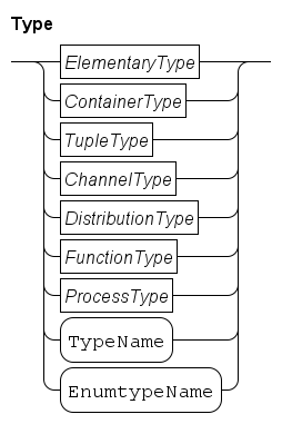
-
The
ElementaryTypeblock contains types that do not build on other types. They are explained further in Elementary types. -
The
ContainerTypeblock contains types that can store values of a single other type, the 'list', 'set', and 'dictionary' type. These types are further explained in Container types. -
The
TupleTypeblock describes 'tuples', a type that can hold values of several other types. -
The
ChannelTypeblocks describes communication channels that connect processes with each other, see Channel type for more explanation. -
The
DistributionTypeblock contains the stochastic distribution type, explained in Distribution type. -
The
FunctionTypecan hold a function definition. It allows you to pass a function to a process or another function. It is further explained in Function type. -
The
ProcessTypecan hold a process definition. It allows you to pass a process definition to a another process. It is further explained in Process type.
The TypeName is the name of a type defined with a type definition (explained in Type definitions).
For example:
type lot = real;

model M():
    lot x;

    ...
end
The lot x variable declaration (explained in Local variables) uses the type definition of lot at the first line to define the type of variable x.
The EnumTypeName is similar, except it uses an enumeration definition (see Enumeration definitions) as type.
For example:
enum FlagColours = {red, white, blue};

model M():
    FlagColours x = white;

    ...
end
The FlagColours x variable declaration defines that variable x has the type of the enumeration, and can hold its values.
Elementary types
The elementary types do not depend on other types to define their set of allowed values. They have the following syntax:
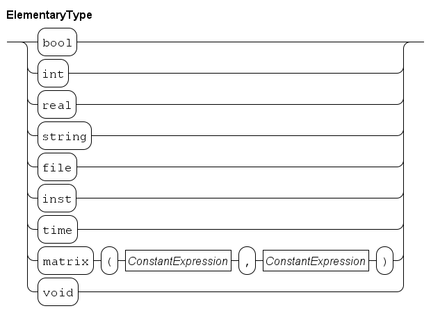
As you can see, they are mostly just a single keyword.
The ConstantExpression nodes in the matrix type line are integer expressions with a fixed (and known) value before execution of the program.
More information about the elementary types is provided below.
Boolean type
The bool keyword denotes the boolean data type.
The allowed values are false and true.
While it is allowed to store boolean values in other data types, their most frequent use is in expressions of statements that decide what to do, for example, the condition in the while, if or select statement (see While loop statement, Choice statement and Select statement).
Expressions with booleans are explained in Boolean expressions.
Integer type
The int keyword denotes the integer data type, integer numbers from 2147483647 to -2147483648 (a standard signed 32 bit number).
Values outside that range give undefined behavior.
Expressions with integers are explained in Integer expressions.
Real type
The real keyword denotes the real number data type, real numbers between 4.94065645841246544e-324 to 1.79769313486231570e+308 positive or negative (a standard 8 bytes IEEE 754 number).
As normal with floating point numbers in computer systems, many values are missing from the above range.
Expect rounding errors with each calculation.
Expressions with real numbers are explained in Real number expressions.
String type
The string keyword denotes strings, sequences of characters.
It contains all printable ASCII characters U+0020 to U+007E, and 'tab' (U+0009) and 'new line' (U+000A).
Expressions with strings are explained in String expressions.
File type
The file keyword denotes a file at the file system of the computer.
It allows reading and writing values of many data types (not all data types can be read or written).
Expressions with files are explained in File handle expressions.
How to work with files is explained in Input and output.
Instance type
The inst keyword denotes an instance type, it can store a running process.
Its use is to check whether the stored process has ended.
The Finish statement gives more details and provides an example.
Timer type
The timer keyword denotes a count-down timer.
Variables of this type measure time that has passed since their initialization.
Expressions with timers are given in Timer expressions, a tutorial about using timers can be found in Timers.
Matrix type
The matrix type takes two constant expressions that define the number of rows and the number of columns of the matrix.
The main purpose of the data type is to allow temporary storage of matrices so they can be passed on to other software.
The Chi language also has expressions to write literal matrices, see Matrix expression for details.
Void type
The void type denotes that no data is involved.
Values of type void do not exist.
The type is allowed at two places in the Chi specification, namely:
-
As data type of synchronization channels. Further explanation can be found at Communication statements and Channel type.
-
As exit type of Model definitions and Process definitions, to express that it may return an exit value from an Exit statement without arguments.
Container types
The main function of container types is to organize and hold a collection of values of another type (the element type). The syntax diagram of the container types is as follows.
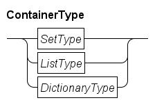
The language has three container types, lists (explained in List type), sets (explained in Set type), and dictionaries (explained in Dictionary type).
List type
The list type has an ordered collection of values from its element type as its value. Duplicate element values are allowed.
The syntax of a list type is given below.
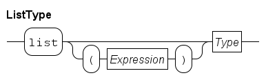
It starts with the keyword list, optionally followed by a parenthesized (non-negative) integer expression denoting the initial number of element values in the collection, and finally the type of the element values.
The default size of the collection is the value of the integer expression, or 0 if there is no such expression. The value of the elements in the initial list value depends on the type of the elements.
A few examples:
list bool    # A list of boolean values, initial value is <bool>[]
list (2) int # A list of integer values, initial value is [0, 0]
For a discussion of operations on values of this type, see List expressions.
Set type
The set type has an unordered collection of values from its element type as its value. Duplicate element values are silently discarded.
The syntax of the set type is given below.
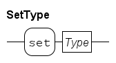
The set type starts with a set keyword, followed by the type of its elements.
Its initial value is the empty set.
An example:
set real # A set of real numbers, initial value <real>{}.For a discussion of operations on values of this type, see Set expressions.
Dictionary type
The dictionary type has an unordered collection of values of its key type, so called keys. The keys are unique in the collection. In addition, the dictionary has a value of its value type associated with each key.
The syntax of a dictionary type is given below.
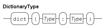
The syntax starts with a dict keyword, and the key type and value type between parentheses, separated by a colon.
The initial value of a dictionary type is the empty dictionary.
An example:
dict (bool : int)  # A dictionary with boolean keys, and integer values.
                   # Initial value <bool:int>{}.
For a discussion of operations on values of this type, see Dictionary expressions.
Tuple type
A tuple contains a fixed number of values of (possibly) different types. It has the following syntax:
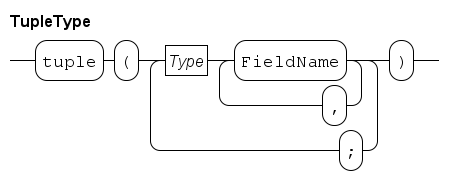
A tuple type starts with the keyword tuple, followed by the list of its fields between parentheses.
Each field has a name and a type.
Sequences of fields with the same type can share their type description, which reduces the amount of text of the tuple type.
Tuple types must have at least two fields.
Examples:
tuple(int a, b)      # A tuple containing fields 'a' and 'b', both of type int
tuple(int a; int b)  # A tuple containing fields 'a' and 'b', both of type int

tuple(lot x; real start) # A tuple with a 'lot' and a 'real' type.
The first two examples are equivalent, the first form is just a bit shorter in notation. The third example is more common fields of different types that are kept together in the modeled system. Expressions with tuples are discussed in Tuple expression.
Channel type
The channel type defines the direction and the type of values transported. The syntax of the channel type is as follows.
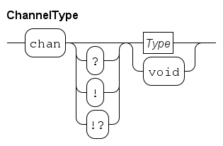
The chan keyword denotes a channel type is being created.
It may be followed by allowed directions of transport, a ! means that sending values is allowed but not for receiving, and a ? means that receiving values is allowed and sending is not allowed.
Finally !? means both sending and receiving is allowed.
The latter is also selected when no direction is specified.
The language silently discards allowed directions.
A channel usable for both sending and receiving may be used as a channel for sending only (dropping the ability to receive at that point).
It does not allow adding directions, a receive-only channel cannot be used for sending.
It can also not be used as a channel for sending and receiving, even if then latter is only used for receiving values (that is, sending is never done).
The type of data that is transported with a communication is given by the Type block.
Signalling channels (that only synchronize without transporting data) are indicated by the void keyword.
The only expressions available for channels are the equality tests, and a function to create new channels, see Channel expressions for details.
Distribution type
The distribution type represents a stochastic distribution. It has the following syntax:
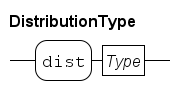
A stochastic distribution allows modeling of random behavior, but with a known chance distribution.
The Type block in the DistributionType diagram defines the type of values drawn.
For a discussion of expressions for the distribution type, see Distribution expressions.
Function type
The function type can hold a function. Its syntax is as follows.
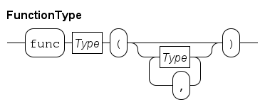
A function type starts with the keyword func followed by the return type of the function and the type of the formal parameters.
The purpose of the function type is to pass functions to processes or other functions, for example, the predicate function in sort and insert, see List functions.
Process type
The process type is similar to the function type (discussed in Function type), except this type can hold a process definition. It has the following syntax:
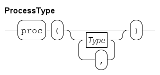
The type starts with the keyword proc followed by the formal parameters of the process definition to store between parentheses.
Expressions with process types are explained in Process expressions.
Lexical syntax
At the lowest level, a Chi specification file consists of a sequence of characters.
The characters are grouped together to form keywords, names, literal values such as numbers, and symbols such as expression operators like + and statement separator ;.
Also comments are recognized at this level.
Whitespace
The characters that delimit groups and lines from each other is known as whitespace. It contains the 'tab' character (U0009), the 'line feed' character (U000A), the 'carriage return' character (U000D), and the 'space' character (U0020).
Comment
A comment is a line of text intended for annotating the program text. It can also be used to (temporarily) add or remove statements. In the latter case, do note that the meaning of the program may change.
A line of comment starts with a 'hash' character #, and continues until a 'line feed' character (or the end of the file).
All characters in the comment are ignored by the simulator.
Names
A name is a word-like group of characters.
It may start with a $ prefix.
After the prefix (if one is provided), first a letter (A to Z or a to z) or an 'underscore' character _ should be used, optionally followed by more letters, 'underscore' characters, or digits 0 to 9.
Some names are special in the sense that the Chi language reserves them for its own use, for example the names model and end.
Keywords are always written using lowercase letters.
In the grammar diagrams, the keywords are shown in a rounded box.
Names starting with a $ prefix are never used as keyword.
Names not used as keyword can be used to give entities in the Chi program a unique identification. In the grammar of this reference manual names are split according to the kind of entity that they refer to:
- ConstantName
-
Name that refers to a constant value, see Constant definitions for details.
- EnumtypeName
-
Name that refers to an enum type, see Enumeration definitions for details.
- EnumvalueName
-
Name that refers to a value within an enum type, see Enumeration value for details.
- FieldName
-
Name that refers to a field in a tuple type, see Tuple type for more details about tuples.
- FunctionName
-
Name that refers to a function definition, see Function definitions for details.
- ModelName
-
Name that refers to a model definition, see Model definitions for details.
- ProcessName
-
Name that refers to a process definition, see Process definitions for details.
- TypeName
-
Name that refers to a type, see Type definitions for details.
- VariableName
-
Name that refers to a variable (see Local variables) or formal parameter in a process or function (see Formal parameters).
Names are also shown in a rounded box, but as shown above, start with an uppercase letter and end with Name.
SVG visualization
The Chi simulator has the possibility to display an SVG file during the simulation. The model can modify the displayed image depending on the state of the simulated system, thus visualizing the system.
Such a visualization is useful for getting a quick global verification, as well as explaining the purpose of the model to people that do not know the detailed ins and outs of the problem being solved.
Below are the technical details of the SVG visualization. The tutorial has a more gentle introduction into the subject.
SVG interface
The SVG visualization itself is controlled by the simulator.
Normally, it is updated just before a time step is performed.
The simulation can however force an update with the redraw command (see below for details).
The simulation accesses the SVG visualization by opening a file for writing with a name like SVG:xyz.svg.
The SVG: prefix redirects the request to the SVG visualizer, the xyz.svg suffix is the name of the SVG file to display.
The file should be available at the file system.
Different Chi processes may open the same file at the same time.
The SVG visualizer can only display one SVG file at a time, it is not allowed for processes to open different .svg files.
Visualization modification commands
After opening the file, the content of the SVG file can be changed by modifying the nodes. This is done by writing lines with commands (one command at each line). Available commands are:
-
Copy an element (recursively)
copy [orig-id], [opt-prefix], [op-suffix], with[orig-id]the id-name of the element to copy,[opt-prefix]an optional prefix that is added to theidof all copied elements, and[opt-suffix]an optional suffix that is added to theidof all copied elements. Since theidof all elements must be unique, leaving both the prefix and the suffix empty gives an error about duplicateidlabels.Note that the element (and its descendants) is only copied, but not moved. In other words, after copying it is fully obscured by the original element. The next step is normally an absolute move command or an attribute command to perform a relative translate transformation.
-
Move an element to an absolute position
absmove [id] ([xpos], [ypos])with[id]the id-name of the element to move,[xpos]the horizontal position to move to, and[ypos]the vertical position to move to. This operation adds a translation to thetransformattribute of the node such that the top-left corner of the bounding rectangle is moved to the provided position. It also takes the existing transformation into account, and in doing so, will fail if the transformation cannot be reversed.The origin of the coordinate system is at the top-left of the SVG visualization window, with positive X running to the right, and positive Y running down.
Avoid using this operation repeatedly on the same element. Instead move it once to a base position, and perform relative translate transformations on a child element to move it to the desired position.
-
Change an attribute of an element
attr [id].[atrribute] = [value]with[id]the id-name of the element,[attribute]the name of the attribute of the element to change, and[value]the new value of the attribute.A change overwrites any previous value of the attribute. Also, names of attributes and syntax of values are not checked.
-
Change the text of an element
text [id] = [value]with[id]the id-name of the element, and[value]the new text. -
Force a redraw of the image
Normally the program redraws the SVG image when it detects a change in time after making changes in the image by using one of the previous commands. With this command you can fake a change in time, thus allowing you to also display intermediate states.
The command is mostly useful in experiments, where time never changes.
Chi Tool Manual
This manual explains how to use the Chi simulation software. Before using the software however, you need to install it. The software is part of the Eclipse ESCET software.
Once you’re finished installing, you can start to simulate Chi programs.
The easiest way to start simulation is to press the F9 key in a Chi text editor, or when a Chi file (a file with a .chi or .chix file extension) is selected in the Project Explorer tab or Package Explorer tab.
Topics
Software operation
The Chi simulator software performs two steps internally:
-
Type checking of the Chi source file, and building a simulator for it.
-
Running the created simulator.
Starting with a .chi source file, both steps have to be performed for a simulation.
As this is the common situation, the software normally combines both steps.
If you run many experiments with the same file, it becomes useful to skip the first step.
How to do this is explained in Compile only.
In addition, the software can be run from the command line.
In that case, command-line options as explained in Command line options need to be specified.
Compile and simulate
Normally, you want to simulate a .chi source file.
The Chi simulator software uses two steps internally (first checking the input and building the simulator, then running the just created simulator), but these steps are combined in the dialog.
The process starts by selecting the source file you want to use (a file with a .chi extension) in the Project Explorer tab or Package Explorer tab, and opening the popup menu with the right mouse button from that selection.
Alternatively, open the file in the editor, and use the right mouse button to get a similar popup menu.
From the popup menu, select Simulate Chi file entry. The selection causes the Console view to be opened in Eclipse, and a dialog window pops up to set the simulator options like below.
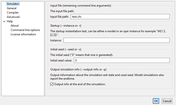
The dialog shows the source file being used in the Input file path box.
Below it, in the Instance box, you can enter how to run the model or the experiment of the source file.
The syntax of the input is the same as you would write it in your Chi file.
For example, with a model definition model M(list real xs, int n): ... end, you could write M([1.5, 2.81], 15) as model instantiation.
If you leave the entry empty, the simulator tries to find an experiment without any parameters (for example X()).
If that fails, it tries to find a model without any parameters (typically M()).
If both attempts fail, or the simulator finds more than one such experiment or model, an error is reported.
If you want to set an initial seed (see Simulating stochastic behavior for a discussion), you can use the Initial seed value box.
Value 0 means 'create a new one'.
This is all you have to do, select OK at the bottom. The software performs its two steps, and if no errors are found, it runs the model.
Quick simulate
For files that do not need any further configuration before they are run, there is a Quick simulate Chi file. This menu option assumes the default configuration (a parameter-less experiment or model needs to be run with a new seed), skips the dialog (saving you from having to press OK) and immediately proceeds with processing the Chi file.
This functionality is also available from the Chi text editor, by pressing the F9 key. Alternatively, you can select a Chi file in the Project Explorer tab or Package Explorer tab, and press the F9 key.
Compile only
The above is convenient for simple experiments, but checking the input and building a simulator each time is tedious if you want to do several experiments with the same source file. For this reason, each step can be done separately as well.
Only building a simulator starts in the same way as above, select a .chi source file from the Project Explorer tab, Package Explorer tab or an editor window, and right-click at it.
Select the Simulate Chi file option from the popup menu.
As the file only gets compiled, the simulator options are of no interest.
Instead switch to the Compiler tab.
It looks like this:
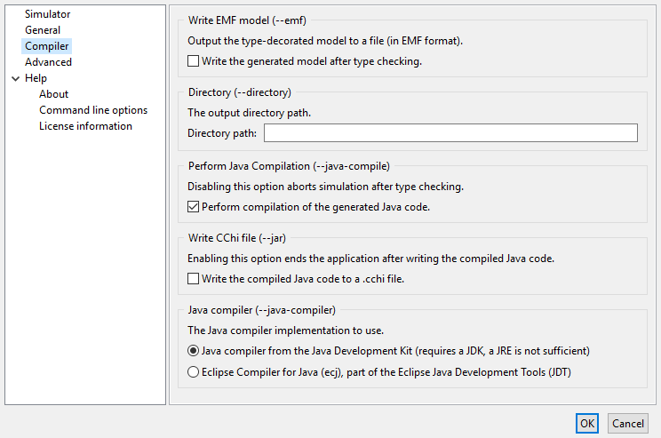
Most settings are only useful for developers, but at the bottom, check the Write the compiled Java code to a .cchi file box, and click OK at the bottom.
Setting this option causes the simulator software to check the input file, build a simulator, write the constructed simulator to a .cchi file (a compiled Chi file), and quit.
No simulation of the Chi model is performed at this time.
Simulate a compiled model
You can simulate the Chi model from the .cchi file now, by selecting that file as source file by right-clicking on it.
Select the Simulate Chi file or the Quick simulate Chi file option as before, and proceed with setting the simulator options and running the model as-if you selected a normal .chi file, as explained in Compile and simulate above.
Terminating a simulation
A simulation ends when:
-
The model goes into a deadlock state,
-
An
exitstatement is performed (see experiments in the tutorial), -
The simulation is terminated by the user, via the console Terminate button (explained below), or
-
A runtime error occurs.
The simulation can be stopped at any time by using the Terminate button (image::./tool-manual/terminate_button.png[]), located at the upper right corner of the console. Note however that if the console does not have the focus, this button may not be visible. If the button is not visible, click somewhere in the console to make the button appear. If even then the button is still not available, it may still appear if you Maximize the console. Also note that the button has no effect while the simulator interactively asks for input from the console. However, once the console input is provided, and Enter is pressed, the termination request will be processed.
Command line options
When you run the Chi software from the command line, the interactive dialog as shown in Software operation is not shown (at least not by default), and everything has to be specified at the command line instead.
The Chi simulator software takes one input file, which is a filename with a .chi, .chix or .cchi file extension.
Below is a list of the available options of such a command line. Most of them are for advanced uses only, and not of interest to most users.
Simulator options
-
--instance=<instance>,-i <instance>Instantiate the model of the file as given by instance. Default is instantiation of a model without parameters.
General application options
-
--help, -hPrints the help text of the application to the console.
-
--option-dialog=<bool>Whether to show the option dialog after the command line options have been processed. Default is
off. -
--output-mode=<outmode>,-m <outmode>The output mode. Specify
errorfor errors only;warningfor errors and warnings only;normal(default) for errors, warnings, and normal output; ordebugfor errors, warnings, normal, and debug output. -
--show-licensePrints the license text of the application to the console.
-
--devmode=<bool>Whether exceptional situations return limited user friendly information (
--devmode=off), or extended developer oriented information (--devmode=on). Default is user friendly information.
Compiler options
-
--emf=<bool>,-e <bool>Whether or not to write the generated EMF model after type checking (default is
off). -
--directory=<dir>,-d <dir>Output directory for generated Java files. Output is not written when the option is empty or not provided.
-
--java-compile=<bool>,-c <bool>Whether or not to perform compilation of the generated Java code (default is
on). -
--jar=<bool>,-j <bool>Whether or not to write the compiled Java simulator classes (default is
off).
Chi release notes
The release notes for the versions of Chi and the associated tools, as part of the Eclipse ESCET project, are listed below in reverse chronological order.
See also the Eclipse ESCET toolkit release notes covering those aspects that are common to the various Eclipse ESCET tools.
Version 11.0 (2026-03-31)
Improvements and fixes:
-
The Chi simulator SVG output now no longer scales on hi-DPI displays on Windows. This prevents severe performance regressions observed in ESCET v10.0. ESCET v10.0 adopted the Eclipse IDE 2025-09, which comes with improved hi-DPI support on Windows, which caused the regressions (issue #1334).
-
The Chi simulator SVG output no longer hangs when showing SVG files with inline images encoded using base64 that contain spaces (issue #1324).
Version 10.0 (2025-12-19)
Improvements and fixes:
-
The Chi simulator SVG visualizer has been fixed for handling of vendor-specific CSS properties starting with a
-, such as Inkscape CSS properties, instyleattributes of SVG elements. Vendor-specific properties are now removed to ensure that the Batik SVG library, used to render SVG images, properly processes the properties that follow the vendor-specific properties (issue #886). -
The Chi simulator SVG visualizer now properly handles and reports CSS rendering errors, similar to SVG XML/DOM errors (issue #888).
-
The Chi documentation no longer contains zero width space characters generated by AsciiDoc, ensuring that there are no undesired line breaks caused by them (issue #1279).
-
The Chi documentation no longer links to
index.htmlin link URLs, but instead now links to the parent that contains theindex.html, resulting in nicer URLs (issue #1317).
Version 8.0 (2025-06-30)
Improvements and fixes:
-
The Chi text editor now has greatly improved performance when the Chi model has many warnings or errors. This may in certain cases also prevent the IDE from freezing indefinitely (issue #995).
-
The Chi simulator can now be started in the ESCET IDE from right click menus of
.chixfiles and editors (issue #1229). -
The Chi simulator documentation now indicates that the simulator can be started from
.chixfiles (issue #1229). -
The Chi tool manual has some small textual improvements (issue #1229).
-
The screenshots of Chi in the ESCET IDE, as part of the Chi documentation and Chi website, have been updated to include the ESCET icon introduced in release v3.0 (issue #1197).
Version 7.0 (2025-03-31)
Improvements and fixes:
-
The Chi website now shows the Chi logo (issue #1140).
Version 0.10 (2023-06-30)
Improvements and fixes:
-
The Chi simulator’s SVG visualizer Save as dialog now properly starts in the directory that contains the SVG file, also on Windows. And it now properly handles paths with spaces and other special characters in them (issue #221).
Version 0.8 (2022-12-21)
Improvements and fixes:
-
Normally,
.chifiles are opened with the Chi text editor. Large files are now however opened with the default non-Chi text editor to avoid performance issues. You can open a file in an editor of your choosing by right clicking it and selecting Open With and then selecting the editor of your choosing, or choosing Other… to open a dialog to choose from a larger selection of editors (issue #199).
Version 0.7 (2022-09-30)
New features:
-
The Chi text editor now has theming support, and comes with a dark theme in addition to the existing light theme. The text editor now automatically uses its dark theme when the Eclipse built-in dark theme is used, and uses a light theme otherwise. The text editor theming behavior can be configured via the Eclipse Preferences dialog (issue #347).
Improvements and fixes:
-
The Chi text editor light theme’s default color has changed from a near-black slightly-brown color to pure black (issue #347).
Version 0.6 (2022-07-07)
Improvements and fixes:
-
Links in the documentation to non-Chi ESCET documentation webpages now use version-specific URLs (issue #386).
-
Improved bibliography references in documentation (issue #365).
-
The issue numbers in the release notes now link to the corresponding GitLab issue (issue #396).
-
Small website style improvements (issue #367).
Version 0.4 (2021-12-17)
Improvements and fixes:
-
Introduced a brand new website (issue #35).
-
Many website URLs have changed due to various website structure changes (issues #35 and #73).
-
Various documentation/website textual improvements, style improvements and other changes (issues #35, #54, #236 and #248).
-
The Chi simulator SVG visualizer functionality to save the image as an SVG file no longer crashes (issue #205).
-
The Chi simulator SVG visualizer functionality to save as an image no longer asks duplicate overwrite questions (issue #223).
-
The Chi simulator no longer crashes when showing an SVG visualizer if the SVG file can’t be loaded (issue #207).
Version 0.3 (2021-10-01)
Improvements and fixes:
-
The website and Eclipse help now use multi-page HTML rather than a single HTML file, although the website still contains a link to the single-page HTML that allows easily searching the full documentation (issue #36).
-
Enabled section anchors for documentation on the website, and disabled section anchors for Eclipse help (issue #36).
-
Several small documentation fixes and improvements (issues #36 and #166).
Version 0.2 (2021-07-07)
Improvements and fixes:
-
Chi simulator no longer crashes when using the Eclipse Compiler for Java (ecj) as Java compiler (issue #46).
Legal
The material in this documentation is Copyright (c) 2010, 2026 Contributors to the Eclipse Foundation.
Eclipse ESCET and ESCET are trademarks of the Eclipse Foundation. Eclipse, and the Eclipse Logo are registered trademarks of the Eclipse Foundation. Other names may be trademarks of their respective owners.
License
The Eclipse Foundation makes available all content in this document ("Content"). Unless otherwise indicated below, the Content is provided to you under the terms and conditions of the MIT License. A copy of the MIT License is available at https://opensource.org/licenses/MIT. For purposes of the MIT License, "Software" will mean the Content.
If you did not receive this Content directly from the Eclipse Foundation, the Content is being redistributed by another party ("Redistributor") and different terms and conditions may apply to your use of any object code in the Content. Check the Redistributor’s license that was provided with the Content. If no such license exists, contact the Redistributor. Unless otherwise indicated below, the terms and conditions of the MIT License still apply to any source code in the Content and such source code may be obtained at https://www.eclipse.org.
Third Party Content
The Content includes items that have been sourced from third parties as set out below. If you did not receive this Content directly from the Eclipse Foundation, the following is provided for informational purposes only, and you should look to the Redistributor’s license for terms and conditions of use.
-
Font Awesome
The Content includes parts of Font Awesome. Font Awesome is licensed under the SIL Open Font License 1.1.
SPDX-License-Identifier: OFL-1.1
-
Highlight.js
The Content includes parts of highlight.js. Highlight.js is licensed under the BSD 3-Clause License.
SPDX-License-Identifier: BSD-3-Clause
-
MathJax
The Content includes parts of MathJax. MathJax is licensed under the Apache License, Version 2.
SPDX-License-Identifier: Apache-2.0
-
Wikipedia external link icon
The Content includes the Wikipedia external link icon. The external link icon is licensed under the Creative Commons Attribution 4.0 International license.
SPDX-License-Identifier: CC-BY-4.0