TRACE Runtime verification

The TRACE tool provides a domain-specific language to formally specify properties about traces. Given such a formal specification and a trace, the TRACE tool can compute whether the trace satisfies the specification. This is a form of (offline) runtime verification. Such verification is broadly applicable: from model validation and verification to diagnosis of problems that occur in a deployed system.

The specifications are stored in plain text files with the etl extension. When such files are opened in the Eclipse UI (with the TRACE feature installed), a dedicated editor is opened with syntax highlighting and support for auto-completion.

Note that TRACE currently does not have algorithms for online runtime verification.

Specifying properties

The language and algorithms are based on temporal logic theory and work on events, claims and signals; dependencies are out of scope. Properties about events and claims can be specified and verified using metric temporal logic (MTL) techniques. Signal temporal logic (STL) can be used to specify and verify properties of signals. These can also be mixed resulting in a top-level MTL formula with STL and MTL subformulas.

MTL atomic propositions

At the basis of MTL formulas are the so-called atomic propositions which are key-value mappings, with an optional indication whether the atomic proposition concerns the start or end of a claim. There is a straightforward evaluation function that indicates whether an atomic proposition is satisfied by a claim or event. This function just checks whether every key-value pair in the atomic proposition is also present in the key-value pairs of the claim or event. The MTL atomic propositions are given by the following syntax:

MtlAp: ('start' | 'end')? AttributeFilter AttributeFilter : '{' KeyVal (',' KeyVal)* '}' KeyVal: IdString '=' IdString IdString: STRING | ID | STRING '+' ID | ID '+' STRING | STRING '+' ID '+' STRING;

For example, the following are MTL atomic propositions:

{ 'name'='A' } { 'name'='A', 'id'=i } end { 'name'='A' }

The first atomic proposition is satisfied by any claim or event with an attribute 'name' with value 'A'. The third is satisfied only by end events of claims which have a 'name' attribute with value 'A'. The second atomic proposition is parameterized and its satisfaction depends on the value of the parameter i. Below we explain how such parameters are defined. Note that the '+' in the 'IdString' rule means concatenation of strings.

STL atomic propositions

At the basis of STL formulas are STL atomic propositions. An STL atomic proposition is a reference to a signal definition, possibly taking the time derivative, and a comparison with a real number. A signal definition consists of a unique identifier, and a signal specification. A signal specification can take several forms:

An attribute filter can be used to select a single signal from the trace (if the filter matches multiple signals, then an error is raised).
A throughput, latency or wip signal can be derived from the trace data (see here) and used in an STL atomic proposition. Note that the throughput is either based on an identifier, or on an MTL atomic proposition which specifies a subset of events to compute the throughput from.
A resource-usage signal (the claimed amount or the number of concurrent clients on a resource) can be derived from the trace data (see here) and used in an STL atomic proposition.

In the latter two types, the derived signals, the signal can be modified with a convolution specification. This computes a signal that gives a sliding-window average of the original signal.

STL atomic propositions are defined with the following syntax:

Some examples of signal definitions are below:

signal s1 : {'name'='signal 1'} signal tp_hr_10s : throughput of id per hr over 10.0 s signal ram_usage : resource-amount {'resource name'='RAM', 'unit'='MB'}

The first signal definition refers to a signal from the trace data which has an attribute 'name' with value 'signal 1'. If this filter does not match exactly one signal, then an error is raised. The second signal definition is the derived identifier-based throughput signal for the identifier 'id'. The throughput is given in units per hour, and averaged over a sliding window of 10 seconds. The third definition computes the instantaneous resource usage of the resource with attributes 'resource name' and 'unit' with values 'RAM' and 'MB' respectively. Using these signal definitions, we can specify the following STL atomic propositions:

d s1 / dt <= 23.3 tp_hr_10s >= 100.0 ram_usage <= 256

Note that the first atomic proposition takes the time derivative of signal s1.

Temporal-logic formulas, definitions and checks

Using the atomic propositions as building blocks, we can specify more complicated formulas. There are two top-level concepts for this: (i) definition, and (ii) checks. Definitions are abbreviations for (parameterized) formulas. Checks are used to specify formulas that need to be verified. Since we can have parameters in MTL atomic propositions and definitions, a check has an optional 'forall' part that specifies the name and domain of an integer parameter. Clearly, if the formula is parameterized, then the forall construct must be used to select parameter values.

Formulas, that can be used in definitions and checks, are based on the MTL and STL atomic propositions explained above. These building blocks can be combined with the following constructs:

not φ : creates the negation of φ
if φ₁ then φ₂, φ₁ and φ₂, φ₁ or φ₂ : creates the boolean combination of the two formulas
globally φ : states that φ holds always from now
finally φ : states that φ eventually holds starting from now
during I φ : states that φ holds during the specified time interval I, relative to now
within I φ : states that φ holds somewhere in the specified time interval I, relative to now
until φ₂ we have that φ₁ : states that φ₁ holds from now until φ₂ holds
by I φ₂ and until then φ₁ : states that φ₁ holds until φ₂ holds and that φ₂ holds within I time units from now

Furthermore, a (parameterized) reference to a definition is also a formula. This all is specified by the following syntax.

Formulas that only contain MTL atomic propositions are MTL formulas. Similarly, formulas that only contain STL atomic propositions are STL formulas. Our variant of STL has the limitation that the general until (the until... and by... constructions above) is not supported. If these constructions are used with two STL subformulas, then the resulting formula will be an MTL formula. Finally, if a formula that uses two subformulas is used, and one of the subformulas is MTL and the other is STL, then the formula will be an MTL formula. In that case, the signal of the STL formula is sampled on the timestamps at which events take place. This can cause unexpected semantic effects. The final section below explains this by an example. For details we refer to [5] of the references.

The syntax above allows us to specify, for instance, the following definitions:

def start_or_end_of_claim_A : { 'name'='A' } def start_or_end_of_claim_A_instance(i) : { 'name'='A', 'id'=i } def end_claim_A : end { 'name'='A' } signal tp_hr_10s : throughput of id per hr over 10.0 s def good_productivity : tp_hr_10s >= 20.0

These definitions are formulas themselves and can be used as such. Examples of checks are the following:

check c1 : finally start_or_end_of_claim_A check c2 : forall ( i : 0 ... 9 ) finally start_or_end_of_claim_A_instance(i)

The first check is true if the trace contains at least one event with attribute 'name' and value 'A'. The second check is true if the trace contains at least one event with attribute 'name' with value 'A', and attribute 'id' with value i for all 0 ≤ i ≤ 9.

Note that the definitions can be used to decompose complicated specifications. By naming them properly, the top-level specification, the check, can be made comprehensible for non-experts. Of course, the specification itself and the decomposition still is specialized work.

Let us now consider the running example. We have an execution trace for the processing of 200 objects that only contains claims with two attributes: the name of the processing step and the identifier (an integer) of the object that is being processed. We specify that the object processing latency is at most 50 ms as follows.

def processing_starts(i) : start { 'name'='A', 'id'=i} def processing_ends(i) : end {'name'='G', 'id'=i} check latency_antecedent : forall (i : 0 ... 199) finally processing_starts(i) check latency_discrete : forall (i : 0 ... 199) globally if processing_starts(i) then within [0.0, 50.0) ms processing_ends(i)

Note that the 'latency_antecedent' check is a sanity check that ensures that the antecedent of the implication in 'latency_discrete' actually occurs in the trace. This example shows that by choosing proper labels for definitions, the resulting checks can be rather readable.

The specifications above are all based on MTL. Below follow examples using STL:

signal tp_per_s : throughput of id per s over 10.0 ms signal work_in_progress : wip of id signal latency_ms : latency of id in ms def work_done_within_100ms : during [100.0, Infty) ms work_in_progress == 0.0 check latency_cont : globally latency_ms <= 50.0 check pipeline_depth : within [0.0, 100.0) ms globally ( work_in_progress >= 3.0 or work_done_within_100ms ) check productivity: within [0.0, 100.0) ms globally ( tp_per_s >= 100.0 or work_done_within_100ms )

The first check is based on the continuous latency signal and states that the latency is never larger than 50 ms. The second check states that after 100 ms of start-up time there are always at least 3 images being processed by the system, except when the system is stopping. This pattern to deal with transient behavior during start up and shut down is also used in the third check to state that the steady-state throughput is at least 100 frames per second.

A method for creating formulas

Creating proper formulas is generally not straightforward. Below we describe a top-down method to systematically develop a formula.

1. Write down the top-level formula in semi-natural language

The first step is to write down the formula that needs to be checked in semi-natural langage. Try to formulate it using the following constructs:

It must always hold that ... / during [] it always holds that ...
Eventually ... happens / within [] ... happens
Until ... we have that ... / by [] ... and until then ...

Here the ... are so-called sub-formulas that can be defined later. The [] indicate time intervals. Note that the second variations in the items above are specializations of the first versions; they add a specific time constraint. It usually helps if you can write the sub-formulas also in semi-natural language. Examples are the following:

It must always hold that the throughput is at least 100 wafers per hour.
Within 10 seconds a wafer change happens.
Until measurements have been done we have that no pickup activity happens.

Using the specification language, these sentences can be partially formalized. Below is the formalization of the first check. Note that we have applied the globally operator, and introduced a definition (which still is not complete) for the sub-formula about the throughput.

def throughput_is_at_least_than_100_wafers_per_hour : ... check c1 : globally throughput_is_at_least_than_100_wafers_per_hour

The formalization of the second check is as follows (note the formalization of the time interval):

def a_wafer_change_happens : ... check c2 : within [0.0, 10.0] s a_wafer_change_happens

The third check is formalized as follows:

def no_pickup_activity_happens : ... def measurements_have_been_done : ... check c3 : until measurements_have_been_done we have that no_pickup_activity_happens

2: Complete definitions

The top-level checks have been defined now in terms of definitions that are not yet formalized. This step makes these definitions formal by repeatedly applying it until no informal definitions are left. Again, we first decompose with semi-natural language. We can use the following patterns:

Event ... occurs
Signal ... has value larger/smaller/equal than/to ...
If ... then ...
... and ...
... or ...
not/no ...
It must always hold that ... / during [] it always holds that ...
Eventually ... happens / within [] ... happens
Until ... we have that ... / by [] ... and until then ...

We use the third check above as an example:

def no_pickup_activity_happens : no pickup event occurs def measurements_have_been_done : a measurement done event occurs and within 10 ms another such event occurs check c3 : until measurements_have_been_done we have that no_pickup_activity_happens

We first formalize that "no pickup event occurs". We introduce another definition for the pickup event (a MTL atomic proposition), and use the not construction:

def pickup_event : { 'name'='pickup' } def no_pickup_activity_happens : not pickup_event def measurements_have_been_done : a measurement done event occurs and within 10 ms another such event occurs check c3 : until measurements_have_been_done we have that no_pickup_activity_happens

The measurements_have_been_done definition then is formalized as follows.

def pickup_event : { 'name'='pickup' } def no_pickup_activity_happens : not pickup_event def measurement_done_event : { 'name'='measure', 'type'='done' } def measurements_have_been_done : ( measurement_done_event and within (0.0, 10.0] ms measurement_done_event ) check c3 : until measurements_have_been_done we have that no_pickup_activity_happens

Note the subtlety with respect to the interval (0.0, 10.0], which is a left-open interval. This is needed to exclude the first measurement event. A single measurement event would satisfy the measurements_have_been_done formula if the interval is left-closed, i.e., [0.0, 10.0].

Although this specification is complete, it is not exactly the right one. It does not exclude the situation where a pickup event happens between the two measurement events. This is allowed, because the measurements_have_been_done formula is true at the moment of the first of the measurement events. This is the nature of the temporal operators, that can only look into the future. To fix this, we need to exclude pickup activity also between the two measurement events. We therefore change the "within" operator to the "until" operator, and rename our definition slightly:

def pickup_event : { 'name'='pickup' } def no_pickup_activity_happens : not pickup_event def measurement_done_event : { 'name'='measure', 'type'='done' } def measurement_without_pickup_activity : ( measurement_done_event and by (0.0, 10.0] ms measurement_done_event and until then no_pickup_activity_happens ) check c3 : until measurement_without_pickup_activity we have that no_pickup_activity_happens

3: Rewrite to improve readability

The final step is to rewrite the definitions to improve the readability. Sometimes it helps to introduce additional definitions, or to merge definitions. Also naming the definitions in a way such that semi-natural language appears is a good way to increase readability and convey the ideas to others.

Verifying execution traces

Above we have briefly explained how specifications can be written. Now we show how we can verify such a specification on a given trace in the UI. This can be done by invoking the menu item on a trace view, which opens a dialog to select a specification file with the etl extension from the Eclipse workspace. All checks from the specification are verified and the results are shown in a separate view, see Figure 1.

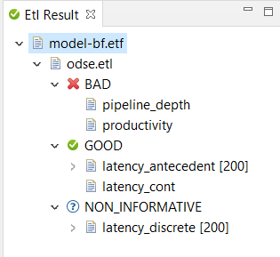
The view keeps track of all trace file and specification combinations that have been checked. If files are modified, then results relating to these files are removed from the result view. Note that a check can have three kinds of results: GOOD, BAD or NON_INFORMATIVE. The last result is only possible when a pure MTL formula is checked (i.e., no continuous signals are used). Then the trace is interpreted as being a prefix of a longer trace that we don't know yet. The NON_INFORMATIVE result then means that from the prefix we cannot decide whether any extension of the prefix will satisfy or dissatisfy the formula. For more information on this informative prefix semantics of MTL we refer to [3] of the references.

Double-clicking a BAD check in the result view adds claims and/or events to the trace to explain why the check is not satisfied. The validity of the check element and each def element that is used in the check is shown either as a colored bar (in case of an STL formula) or as a number of colored events (in case of a pure MTL formula). These elements are either green or red, indicating the validity of the check or def at that point in time. 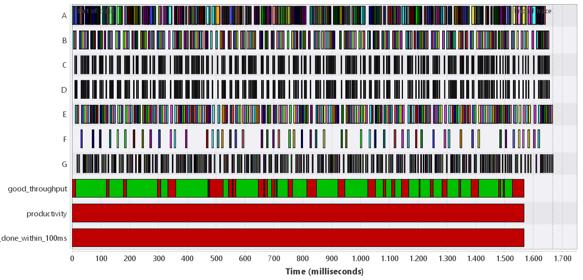For instance, Fig. 2 shows the explanation of the productivity check of the running example that is defined as follows:

signal work_in_progress : wip of id signal tp_per_s : throughput of id per s over 10.0 ms def work_done_within_100ms : during [100.0, Infty) ms work_in_progress == 0.0 def good_throughput: ( tp_per_s >= 100.0 or work_done_within_100ms ) check productivity: within [0.0, 100.0) ms globally good_throughput

The two defs and single check are shown, and clearly the check is not satisfied because there is no continuous good_throughput after 100 ms. This is shown by the red interruptions in the good_throughput section, which indicates that at those points in time the throughput is not good (i.e, at least 100 objects per second).

Figure 2: Explanation of unsatisfied checks.

Mixing MTL and STL formulas

Although the examples above either are pure MTL or pure STL formulas, the MTL and STL concepts can be mixed. This allows specification of properties based on both discrete events and continuous signals. Care has to be taken, however, as the mixed semantics can have counter-intuitive effects.

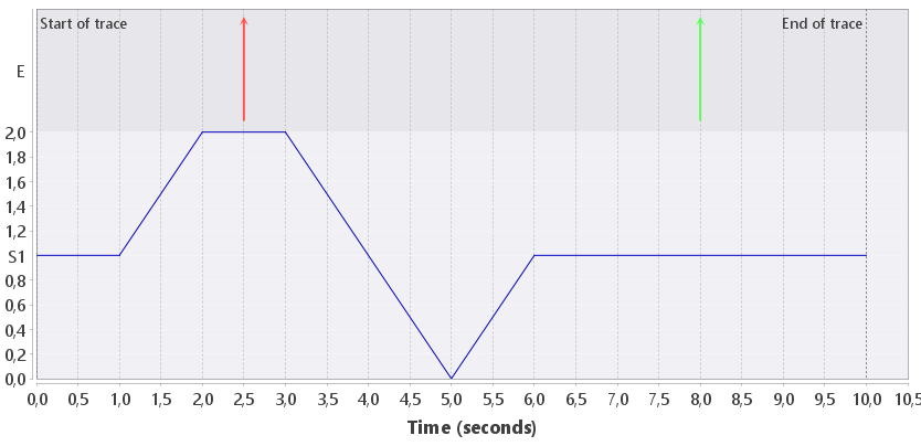
Figure 3: Small example to illustrate mixed semantics.

Consider the execution trace in Figure 3. It consists of two events and a continuous signal. We have the following specification:

def red : {'name'='E', 'color'='red'} def green : {'name'='E', 'color'='green'} signal s1 : {'signal'='S1'} check c1 : globally if s1 >= 1.5 then finally green check c2 : globally if s1 <= 0.5 then finally red check c3 : globally if s1 <= 0.000005 then finally red

The two definitions and the signal declaration are used to refer to the red event, green event and the blue signal respectively. Note that all three checks use both MTL and STL atomic propositions. Now look at check c1. It states that it always holds that if the blue signal is at least 1.5, then a green event eventually happens. On the interval [1.5, 3.5] we have that the antecedent of the implication holds. Therefore, the consequent (a green event) must happen after time 1.5. Clearly this is true. Indeed, verification shows that property c1 holds on the trace.

Now look at check c2. It states that it always holds that if the blue signal is at most 0.5, then a red event eventually happens. The antecedent is true between 4.5 and 5.5 seconds, but no red event follows. Thus, the property should not hold. Indeed, verification shows that property c2 does not hold on the trace.

Finally, consider check c3. This check only differs from c2 in the threshold of the signal. Since the signal reaches value 0 at time 5, the antecedent of the implication is true in a small time interval around 5 seconds. Thus, the property should not hold. Verification, however, shows that property c3 holds on the trace, which is not as expected.

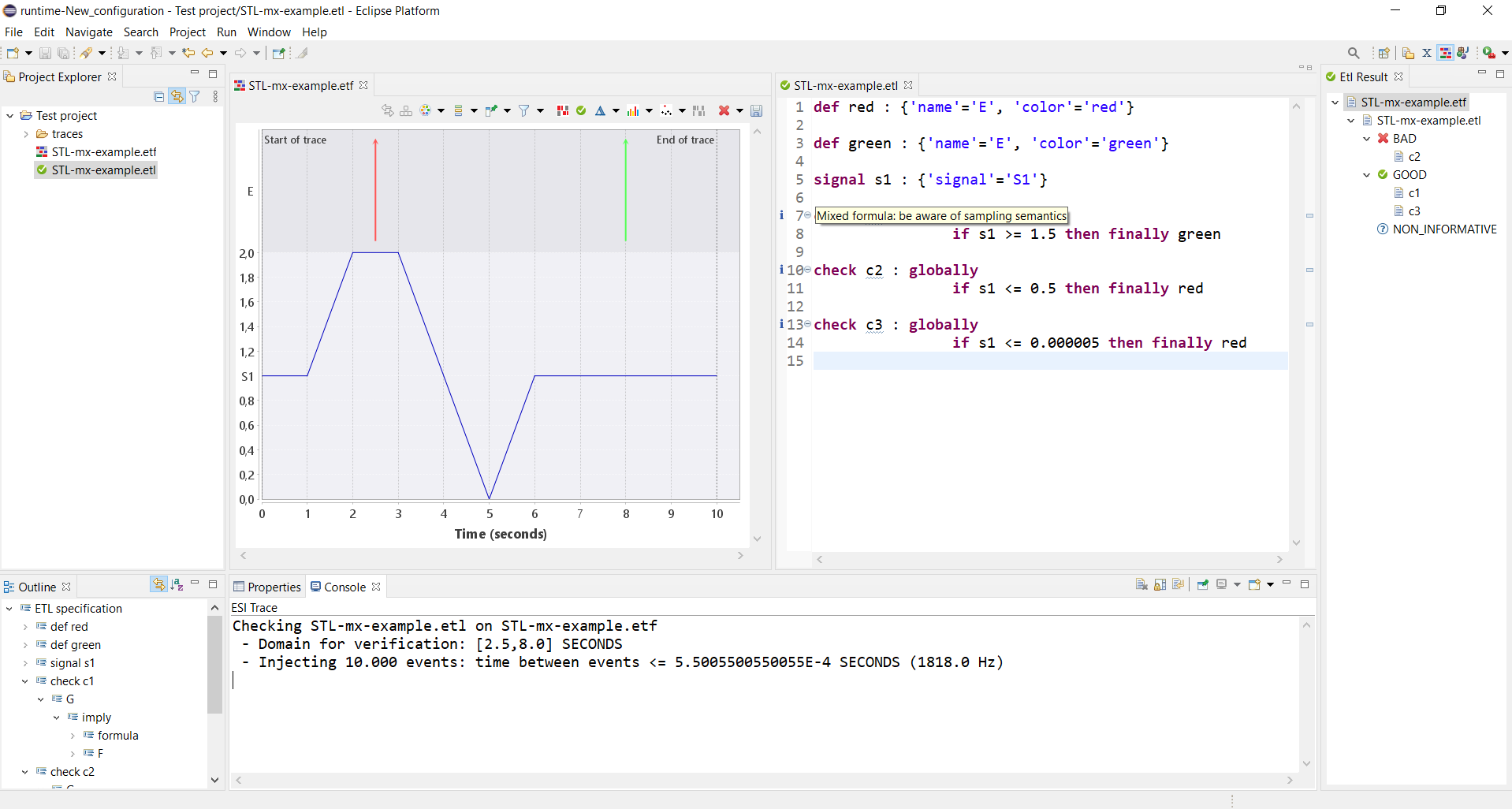
The reason that the verification algorithm concludes that c3 holds is the following. Since a mixed formula is used, the STL subformulas are sampled at the points in time where events occur. Our trace has only two events on the interval [2,8]. Clearly, the events in the discrete part can be very sparse, and therefore the algorithm currently injects a fixed number of dummy events (without attributes) between the first and last event of the trace. This increases the sampling frequency for the STL subformulas, but clearly reduces scalability. (Currently, 10.000 events are injected.) In case of c2, dummy events are injected on the interval where the s1 is at most 0.5, and hence this is seen by the algorithm. This results in the intuitive result that c2 is not satisfied. In case of c3, however, the interval where the antecedent holds is too small: no dummy events are injected in that interval, and hence the algorithm never sees a state where the antecedent of the implication is true. Therefore, the formula is trivially satisfied. This clearly is not as expected, but can be explained by the sampling nature of the algorithm for mixed formulas.

The TRACE tool has two features that makes this complicated semantic behavior more transparent. First, when mixed formulas are specified in the DSL, then a message is shown to the user that warns for the sampling nature that is used for evaluating the formula. Second, when the verification algorithm reports the sampling frequency on the console view. Users can use this to estimate whether the sampling frequency is high enough for their application to see all relevant changes in the signals. Figure 4 shows an image of the TRACE UI with the example explained above. The result view (on the right) shows that c2 is not satisfied and that both c1 and c3 are satisfied. The specification editor has three "i" indications that warn for the sampling semantics if the mouse hovers over them. The console view (bottom) reports the domain on which the verification works, and the number of injected states and the resulting sampling frequency.

Figure 4: TRACE UI with sampling-semantics features.