
Post-Training Quantization with AIDGE#
![]()
What is neural network Quantization ?#
Deploying large neural network architectures on embedded targets can be a difficult task as they often require billions of floating operations per inference.
To address this problem, several techniques have been developed over the past decades in order to reduce the computational load and energy consumption of those inferences. Those techniques include Pruning, Compression, Quantization and Distillation.
In particular, Post Training Quantization (PTQ) consists in taking an already trained network, and replacing the costly floating-point MADD by their integer counterparts. The use of Bytes instead of Floats also leads to a smaller memory bandwidth.
While this process can seem trivial, the naive approach consisting only in rounding the parameters and activations doesn’t work in practice. Instead, we want to normalize the network in order to optimize the ranges of parameters and values propagated inside the network, before applying quantization.
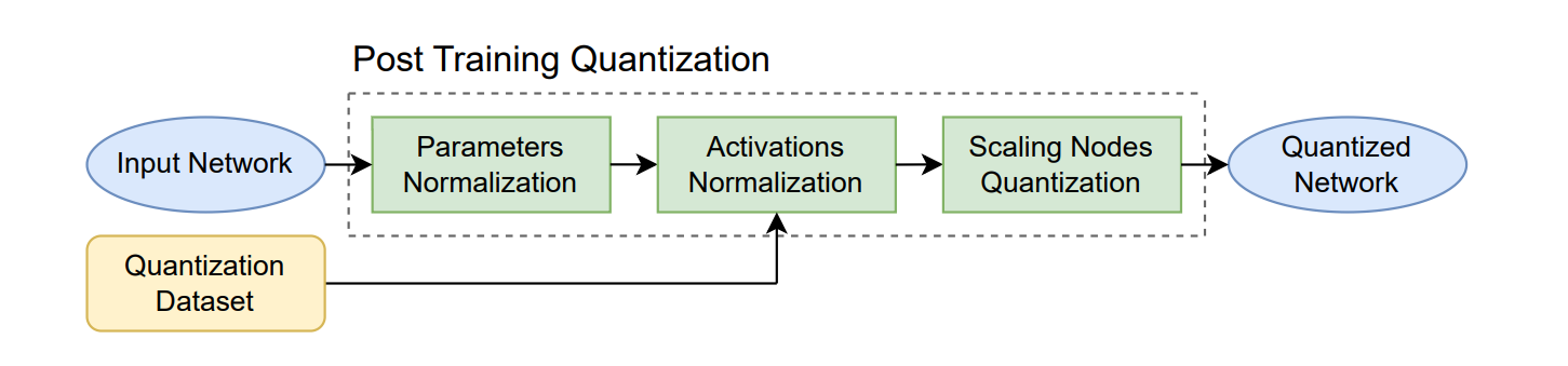
The Quantization Pipeline#
The PTQ algorithm consists of a three-steps pipeline:
First, we optimize the parameter ranges by propagating the scaling coefficients through the network.
Second, we compute the activation values over an input dataset and insert the scaling nodes.
Finally, we quantize the network by reconfiguring the scaling nodes according to the desired precision.
Performing PTQ with AIDGE#
This notebook shows how to perform PTQ of a convolutional neural network, trained on the MNIST dataset.
The tutorial is constructed as follows :
Setup of the AIDGE environment
Loading of the model and running example inferences
Evaluation of the trained model’s accuracy
Post-Training Quantization and test inferences
Evaluation of the quantized model accuracy
As we will observe in this notebook, there is zero degradation in accuracy for an 8-bit PTQ.
Environment setup#
Ensure that the Aidge modules are properly installed in the current environment. If it is the case, the following setup step can be skipped.
Note: When running this notebook on Binder, all required components are pre-installed.
[ ]:
%pip install aidge-core \
    aidge-onnx \
    aidge-backend-cpu \
    aidge-quantization
Import modules#
Besides Aidge modules, we need Numpy for manipulating the inputs, Matplotlib for visualization purposes, and gzip to uncompress the numpy dataset.
Then we want to import the Aidge modules:
the core module contains everything we need to manipulate the graph.
the backend module allows us to perform inferences using the CPU.
the onnx module allows us to load the pretrained model (stored in an onnx file).
the quantization module encaplsulate the Post Training Quantization algorithm.
[ ]:
import gzip
import numpy as np
import matplotlib.pyplot as plt

import aidge_core
import aidge_onnx
import aidge_backend_cpu
import aidge_quantization
import aidge_model_explorer

# The following line only if you want to change default log level
aidge_core.Log.set_console_level(aidge_core.Level.Error)

print(" Available backends : ", aidge_core.Tensor.get_available_backends())
Exploring the original ONNX Model#
Download the ONNX file and Database (if needed)#
If git-lfs is not installed, the model and data can be downloaded using the following code snippet.
Reminder: This step is not needed when running in Binder.
[ ]:
BASE_URL = "https://gitlab.eclipse.org/eclipse/aidge/aidge/-/raw/main/examples/tutorials/PTQ_tutorial/"

# Download the model, input and output data files
files_to_download = ["ConvNet.onnx", "mnist_samples.npy.gz", "mnist_labels.npy.gz"]

for file_name in files_to_download:
    aidge_core.utils.download_file(
        file_path=file_name, file_url=f"{BASE_URL}{file_name}"
    )
Setup variables and Database visualization#
Then, let’s define the configurations of this script …
[ ]:
NB_SAMPLES = 100
Now, let’s load and visualize some samples:
[ ]:
samples = np.load(gzip.GzipFile("mnist_samples.npy.gz", "r"))
labels = np.load(gzip.GzipFile("mnist_labels.npy.gz", "r"))
[ ]:
for i in range(10):
    plt.subplot(1, 10, i + 1)
    plt.axis("off")
    plt.tight_layout()
    plt.imshow(samples[i], cmap="gray")
Importing the model in Aidge#
[ ]:
aidge_model = aidge_onnx.load_onnx("ConvNet.onnx")
aidge_core.remove_flatten(aidge_model)  # we want to get rid of the 'flatten' nodes ...
Setting up the Aidge Scheduler#
In order to perform inferences with Aidge we need to setup a Scheduler. But before doing so, we need to create a data producer node and connect it to the network.
[ ]:
# Set up the backend
aidge_model.set_datatype(aidge_core.dtype.float32)
aidge_model.set_backend("cpu")

# Create the Scheduler
scheduler = aidge_core.SequentialScheduler(aidge_model)
Running some example inferences#
Now that the scheduler is ready, let’s perform some inferences. To do so we first declare a utility function that will prepare and set our inputs, propagate them and retrieve the outputs.
[ ]:
def propagate(model, scheduler, sample, aidge_dtype=aidge_core.dtype.float32):
    # Setup the input
    sample = np.reshape(sample, (1, 1, 28, 28))
    input_tensor = aidge_core.Tensor(sample)
    input_tensor.to_dtype(aidge_dtype)

    # Run the inference
    scheduler.forward(True, [input_tensor])
    # Gather the results
    output_node = model.get_ordered_outputs()[0][0]
    output_tensor = output_node.get_operator().get_output(0)
    return np.array(output_tensor)


print("\n EXAMPLE INFERENCES :")
for i in range(10):
    output_array = propagate(aidge_model, scheduler, samples[i])
    print(labels[i], " -> ", np.round(output_array, 2))
Computing the original model accuracy#
[ ]:
def compute_accuracy(model, samples, labels, aidge_dtype=aidge_core.dtype.float32):
    acc = 0
    for i, x in enumerate(samples):
        y = propagate(model, scheduler, x, aidge_dtype)
        if labels[i] == np.argmax(y):
            acc += 1
    return acc / len(samples)


accuracy = compute_accuracy(aidge_model, samples[0:NB_SAMPLES], labels)
print(f"\n MODEL ACCURACY : {accuracy * 100:.3f}%")
Model Visualization Before PTQ#
aidge_model_explorer, which displays the model as a graph in the browser.[ ]:
aidge_model_explorer.visualize(aidge_model, "model_before_ptq")
Quantization dataset creation#
We need to convert a subset of our Numpy samples into Aidge tensors, so that they can be used to compute the activation ranges.
[ ]:
tensors = []
for sample in samples[0:NB_SAMPLES]:
    sample = np.reshape(sample, (1, 1, 28, 28)).astype(np.float32)
    tensor = aidge_core.Tensor(sample)
    tensors.append(tensor)
Fake or True Quantization ?#
With Aidge, it’s possible to perform two types of quantification : Fake or True Quantization.
Clamped to the quantization range (e.g., [-128, 127] for int8)
Rounded to the nearest representable integer level
This process allows you to:
Evaluate quantization effects on model accuracy before implementing integer kernels
Debug quantization errors while keeping the model in a safe float environment
Train or fine-tune models with quantization awareness (QAT)
Ensure consistency between simulated and real integer inference
In summary, fake quantization is essential for experimenting with new bit widths (such as 4-bit or even lower) and verifying that your quantization scheme preserves model performance, all without requiring specific integer operator implementations.
We may also want to accurately reflect what will happen on the target machine and capture the actual behavior of the kernels with their precision determined by the hardware present. In this case, we would perform True quantization. This would implement the rescaling specification using bitshift (single_shift option), for example, and the casting of the data types being manipulated.
Graph Annotation Before PTQ#
The last step before invoking PTQ is to annotate the graph to specify the desired precision.
There are two possible approaches:
1. Manual Annotation#
The user can manually annotate the graph by adding the dynamic attributes:
quantization.ptq.precisionquantization.ptq.accumulationprecision
to each node in the graph.
⚠️ This method can be tedious and prone to errors.
2. Automatic Annotation#
Alternatively, the user can use the function auto_assign_node_precision() which automatically assigns the desired precisions across the entire graph.
It takes as arguments the target precisions for:
Weights
Activations
Accumulations & Biases
Finally, we still need to define the number of bits for quantizing the model (to properly quantize the inputs) in accordance with the data types selected in the auto_assign_node_precision() function.
[ ]:
NB_BITS = 4
weight_precision = aidge_core.dtype.int4
activation_precision = aidge_core.dtype.int4
bias_and_accumulation_precision = (
    aidge_core.dtype.int16
)  # The precision for the accumulation must always be greater
Set ``NB_BITS`` to the desired value (e.g., 4 for 4-bit quantization) to properly quantize the inputs on that bit width.
Choose the type of quantization with the variable fake_quantize to True (Fake quantization) or False (True quantization). Note that this choice requires mastery of the input data tensor type. Indeed, depending on whether we are using Fake quantization or True quantization, we will have a tensor in float32 or in the integer type expected by the developer.
Adapt the node auto-tagging routine to match the new bit width:
weight_precision = aidge_core.dtype.int4activation_precision = aidge_core.dtype.int4bias_and_accumulation_precision = aidge_core.dtype.int16
Execute PTQ: The model can now be quantized to 4 bits.
Applying PTQ to the model#
With the setup complete, we can run the PTQ routine.
Note: after quantization, the scheduler must be updated.
[ ]:
# This step is to enable the implementation of the two quantifications in the tutorial sequence.
fake_quantize_graph = aidge_model.clone()
true_quantize_graph = aidge_model.clone()
Fake Quantization implementation#
[ ]:
fake_quantize = (
    True  # PTQ selection type: fake quantize (True) or True Quantize (False)
)
in_dtype = aidge_core.dtype.float32

aidge_quantization.auto_assign_node_precision(
    fake_quantize_graph,
    weight_precision,
    activation_precision,
    bias_and_accumulation_precision,
)
[ ]:
aidge_quantization.quantize_network(
    network=fake_quantize_graph,  # The AIDGE model to quantize
    calibration_set=tensors,  # Calibration dataset used to estimate useful value ranges
    clipping_mode=aidge_quantization.Clipping.MSE,  # Clipping method applied (e.g., MSE clipping)
    no_quant=False,  # Debug flag; disables quantization rounding if True to avoid data loss
    optimize_signs=False,  # Sign optimization: can improve post-quantization accuracy
    # by detecting purely unsigned ranges and exploiting them
    single_shift=False,  # Single Shift Approximation:
    # replaces floating-point multiplications with bit shifts
    # Note: only effective for integer target types
    fold_graph=True,  # Apply constant folding to merge quantizers with their producers
    # Reduces graph size and improves efficiency
    fake_quantize=fake_quantize,  # If True, does not cast tensors to the target datatype
    # Graph stays in float (useful for testing or simulation)
    verbose=False,  # Enable verbose logging
)

scheduler = aidge_core.SequentialScheduler(fake_quantize_graph)
fake_quantize argument was not enabled, the model has been cast to the desired target type.[ ]:
aidge_model_explorer.visualize(fake_quantize_graph, "model_after_PTQ")
Performing inference with the fake quantized model#
Now that the network has been quantized, it’s time to evaluate it by running inference. Before doing so, remember that the 8-bit network expects 8-bit inputs. We therefore need to rescale the input tensors accordingly.
[ ]:
scaling = 2 ** (NB_BITS - 1) - 1
for i in range(NB_SAMPLES):
    samples[i] = np.round(samples[i] * scaling)
We can now perform inference using the quantized model.
[ ]:
print("\n EXAMPLE FAKE QUANTIZED INFERENCES :")
for i in range(10):
    input_array = np.reshape(samples[i], (1, 1, 28, 28))
    output_array = propagate(fake_quantize_graph, scheduler, input_array, in_dtype)
    print(labels[i], " -> ", np.round(output_array, 2))
fake_quantize_graph.log_outputs("fake_quant_tensors")
Evaluating the accuracy of the fake quantized model#
As with the original network, we now compute the quantized model’s accuracy:
[ ]:
accuracy = compute_accuracy(
    fake_quantize_graph, samples[0:NB_SAMPLES], labels, in_dtype
)
print(f"\n QUANTIZED MODEL ACCURACY : {accuracy * 100:.3f}%")
True Quantization implementation#
[ ]:
fake_quantize = (
    False  # PTQ selection type: fake quantize (True) or True Quantize (False)
)
in_dtype = activation_precision

aidge_quantization.auto_assign_node_precision(
    true_quantize_graph,
    weight_precision,
    activation_precision,
    bias_and_accumulation_precision,
)
[ ]:
aidge_quantization.quantize_network(
    network=true_quantize_graph,  # The AIDGE model to quantize
    calibration_set=tensors,  # Calibration dataset used to estimate useful value ranges
    clipping_mode=aidge_quantization.Clipping.MSE,  # Clipping method applied (e.g., MSE clipping)
    no_quant=False,  # Debug flag; disables quantization rounding if True to avoid data loss
    optimize_signs=False,  # Sign optimization: can improve post-quantization accuracy
    # by detecting purely unsigned ranges and exploiting them
    single_shift=True,  # Single Shift Approximation:
    # replaces floating-point multiplications with bit shifts
    # Note: only effective for integer target types
    fold_graph=True,  # Apply constant folding to merge quantizers with their producers
    # Reduces graph size and improves efficiency
    fake_quantize=fake_quantize,  # If True, does not cast tensors to the target datatype
    # Graph stays in float (useful for testing or simulation)
    verbose=False,  # Enable verbose logging
)

scheduler = aidge_core.SequentialScheduler(true_quantize_graph)
fake_quantize argument was not enabled, the model has been cast to the desired target type.[ ]:
aidge_model_explorer.visualize(true_quantize_graph, "model_after_PTQ")
Performing inference with the true quantized model#
Now that the model has been quantized, it’s time to evaluate it by running inference. We use previous normalized samples (during fake quantization). We can now perform inference using the quantized model.
[ ]:
print("\n EXAMPLE TRUE QUANTIZED INFERENCES :")
for i in range(10):
    input_array = np.reshape(samples[i], (1, 1, 28, 28))
    output_array = propagate(true_quantize_graph, scheduler, input_array, in_dtype)
    print(labels[i], " -> ", np.round(output_array, 2))
true_quantize_graph.log_outputs("true_quant_tensors")
Evaluating the accuracy of the true quantized model#
As with the original network, we now compute the quantized model’s accuracy:
[ ]:
accuracy = compute_accuracy(
    true_quantize_graph, samples[0:NB_SAMPLES], labels, in_dtype
)
print(f"\n QUANTIZED MODEL ACCURACY : {accuracy * 100:.3f}%")
Task completed!#
We observe that 8-bit Post-Training Quantization does not degrade the model’s accuracy. This result demonstrates that a well-designed quantization algorithm can enable the deployment of neural networks on resource-constrained devices, where operating with bytes is optimal.Feel free to experiment by re-running this notebook with even more aggressive quantization settings!