Coordinate systems and formulary

This chapter serves as an introductory reference guide for SCM. It shows the definitions of the coordinate systems, which are used and required by the model, and their transformations (see Coordinate systems). Subsequently, a formulary for frequently used calculations within the model is given (see Formulary).

Coordinate systems

There are three coordinate systems, which are used by SCM:

Inertial coordinates
Road coordinates
Vehicle coordinates

The inertial system (also called world system) is a stationary, planar, Cartesian coordinate system, which is defined by its two coordinates x and y.

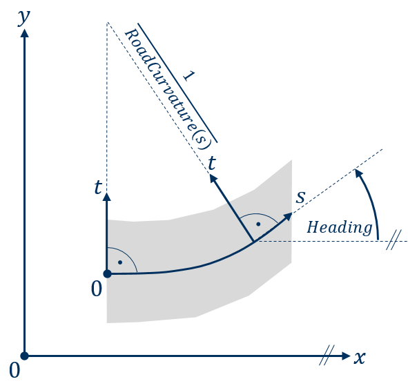
The road system is a stationary, planar, path coordinate system, which is defined within the inertial system by drawing a curvature progression RoadCurvature(s) (inverse of the curve radius) along its path coordinate s (see Fig. 42). This results in two additional system-related coordinates:

Lateral coordinate t (always orthogonal to the path coordinate s)
Angle of orientation Heading (torsion of the local path coordinate s towards the inertial coordinate x)

Fig. 42 Definition of the road system in reference to the inertial system

The vehicle system is a body-fixed, planar, Cartesian coordinate system, which is defined by the vehicle’s longitudinal axis Lon and lateral axis Lat. Its orientation is defined by:

the angle Yaw towards the inertial coordinate x
the angle RelativeYaw towards the road coordinate s

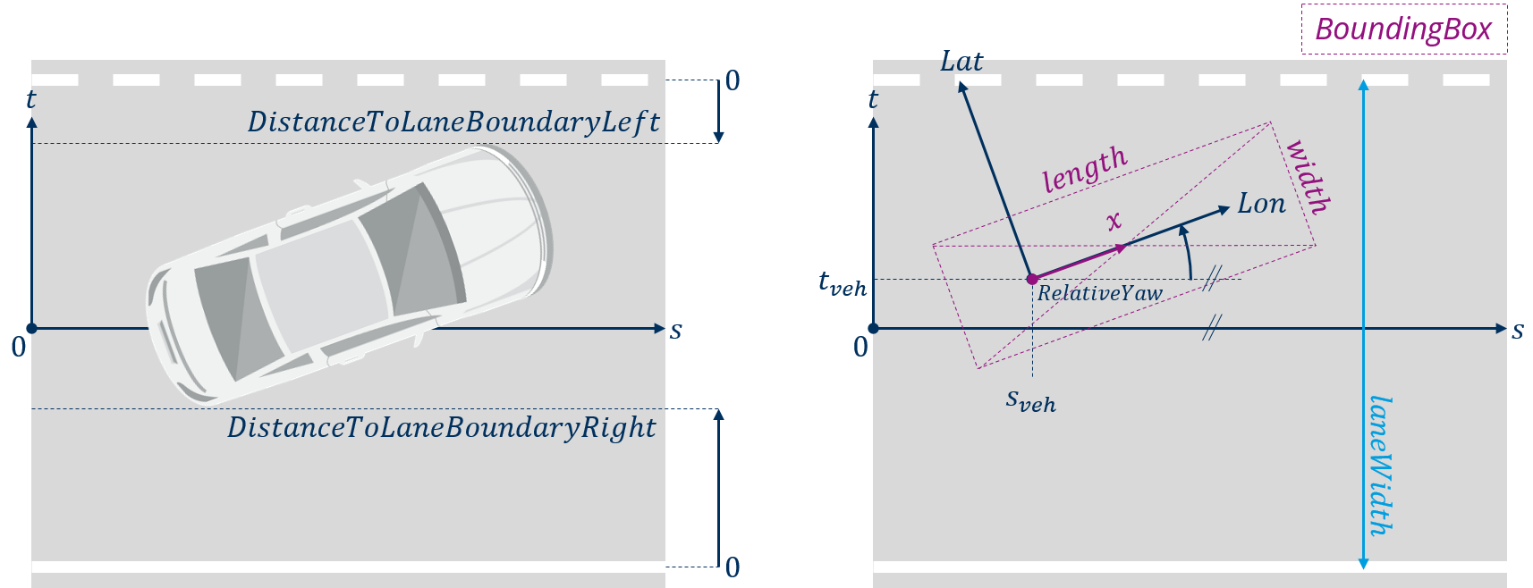
The point of reference for an agent, i.e. the origin of the vehicle system, is set in the centre of the rear axle, but the MainLocatePoint, which is primarily used for the lane assignment of an agent, is set in the centre of the vehicle’s front-bumper (see Fig. 43).

Fig. 43 Definition of the vehicle system in reference to the inertial (left) and road system (right)

The calculations for the transformation of these three coordinate systems are given subsequently.

Transforming road to inertial coordinates

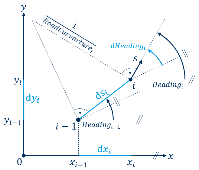
The road system is defined within the inertial system by drawing a curvature progression RoadCurvature(s) (inverse of the curve radius) along its path coordinate s. In mathematical terms, this constitutes a numerical integration over s, which is defined according to the generating system of planar paths by Kramer (Kraftfahrzeugführung: Modelle - Simulation - Regelung, Munich, Carl Hanser, 2008; see Fig. 44).

The incremental change of the path coordinate s between the current integration step i and the previous integration step i – 1 is defined as ds_i. The progression of this increment along the orientation Heading_{i – 1} from the previous step results in incremental changes of the inertial coordinates x and y:

$dx_{i} = cos(Heading_{i – 1}) \cdot ds_{i}$

$dy_{i} = sin(Heading_{i – 1}) \cdot ds_{i}$

The new inertial coordinates are therefore:

$x_{i} = x_{i – 1} + dx_{i}$

$y_{i} = y_{i – 1} + dy_{i}$

The progression of the current RoadCurvature_i along the incremental change ds_i also results in an incremental change dHeading_i of the orientation:

$dHeading_{i} = arcsin(RoadCurvature_{i} \cdot ds_{i})$

The new orientation is therefore:

$Heading_{i} = Heading_{i – 1} + dHeading_{i}$

Transforming vehicle to inertial coordinates

As the vehicle system is body-fixed, the transformation of the position and orientation of a vehicle into stationary coordinate systems can only be realized by means of the equations of motion of the vehicle’s body along the simulation time. The LongitudinalAcceleration along the vehicle’s longitudinal axis Lon (see Fig. 43) is fundamental for the motion of an agent. It is generated by the module DynamicsRegularDriving:

Accelerating due to a driving torque from the powertrain results in a positive LongitudinalAcceleration
Decelerating due to driving resistances or a braking torque from the brake system results in a negative LongitudinalAcceleration

The lateral dynamics of SCM are based on a simple rolling relationship according to Ackermann, i.e. neither tire slip nor external disturbances (e.g. side wind, cross slope) are considered. Therefore, the LateralAcceleration along the vehicle’s lateral axis Lat (see Fig. 43) is defined by the constraint of the centrifugal acceleration:

$LateralAcceleration = LongitudinalVelocity^2 \cdot VehicleCurvature$

The LongitudinalVelocity along the vehicle’s longitudinal axis Lon is defined by the numerical integration of the LongitudinalAcceleration over time:

$LongitudinalVelocity_{i} = LongitudinalAcceleration_{i} \cdot dtime + LongitudinalVelocity_{i – 1}$

The VehicleCurvature of the trajectory, which is drawn by the vehicle’s rear axle, is defined by the Ackermann condition of WheelBase, SteeringWheelAngle, and the overall SteeringRatio of the steering system:

$VehicleCurvature = \frac{tan(\frac{SteeringWheelAngle}{SteeringRatio})}{WheelBase}$

The LateralAcceleration is the result of the centrifugal force, which the vehicle’s body experiences due to cornering and which is countered by the lateral forces of the tires. It is therefore not causing the body’s motion, but it is resulting from it. The representation of the vehicle body’s motion in the inertial system must therefore not be realized by simply integrating LongitudinalAcceleration and LateralAcceleration and vectorising the velocities by means of the Yaw angle. It is also done by numerical integration over time by means of the generating system of planar paths by Kramer (see Transforming road to inertial coordinates). It must thereby be considered that the kinematical lateral acceleration and velocity along the vehicle’s lateral axis Lat is equal to zero, because tire slip is neglected (i.e. the vehicle cannot just slip sideways). Therefore, the above mentioned LongitudinalAcceleration and LongitudinalVelocity of the vehicle system are also equal to the vectorised AbsoluteAcceleration and AbsoluteVelocity of the vehicle’s body:

$AbsoluteAcceleration/Velocity = \sqrt{LongitudinalAcceleration/Velocity^2 + LateralAcceleration/Velocity^2}$

$AbsoluteAcceleration/Velocity = \sqrt{LongitudinalAcceleration/Velocity^2 + 0}$

$AbsoluteAcceleration/Velocity = LongitudinalAcceleration/Velocity$

As the terms LongitudinalAcceleration/Velocity and LateralAcceleration/Velocity are also used to describe accelerations and velocities in the road system (see State variables defined in the road system), AbsoluteAcceleration/Velocity is primarily used for accelerations and velocities caused by powertrain, brake system, or driving resistances.

The incremental change of the vehicle position along its longitudinal position Lon between the current time step i and the previous time step i – 1 is defined as dLon_i:

$dLon_{i} = AbsoluteVelocity_{i} \cdot dtime$

The progression of this increment along the orientation Yaw_{i – 1} from the previous time step results in incremental changes of the inertial coordinates x and y:

$dx_{i} = cos(Yaw_{i – 1}) \cdot dLon_{i}$

$dy_{i} = sin(Yaw_{i – 1}) \cdot dLon_{i}$

The new inertial coordinates are therefore:

$x_{i} = x_{i – 1} + dx_{i}$

$y_{i} = y_{i – 1} + dy_{i}$

The progression of the current VehicleCurvature_i along the incremental change dLon_i also results in an incremental change dYaw_i of the orientation:

$dYaw_{i} = arctan(VehicleCurvature_{i} \cdot dLon_{i})$

The new orientation is therefore:

$Yaw_{i} = Yaw_{i – 1} + dYaw_{i}$

Contrary to the generating system of planar paths for the road system (see Transforming road to inertial coordinates), arctangent is used for the calculation of dYaw_i instead of arcsine here, because VehicleCurvature is defined for the vehicle’s rear axle and not its front axle.

Transforming vehicle to road coordinates

Transforming vehicle coordinates into the road system is very similar to Transforming vehicle to inertial coordinates. The most crucial thing that must be considered is that the road system is not a purely Cartesian coordinate system, but is determined by a RoadCurvature itself. Focus point of the transformation is the angle of orientation RelativeYaw of the vehicle’s body towards the local path coordinate s. The incremental change dRelativeYaw results from the difference between the RoadCurvature and the VehicleCurvature. This difference in curvature results in different local values for the angles of orientation Heading (road) and Yaw (vehicle) towards the inertial system. The incremental change dRelativeYaw is therefore defined by the difference of the incremental changes dYaw and dHeading:

$dRelativeYaw = dYaw – dHeading$

Considering this condition, the transformation can be done by numerical integration over time by means of the generating system of planar paths by Kramer (see Transforming road to inertial coordinates). The incremental change of the vehicle position along its longitudinal position Lon between the current time step i and the previous time step i – 1 is defined as dLon_i:

$dLon_{i} = AbsoluteVelocity_{i} \cdot dtime$

The progression of this increment along the orientation RelativeYaw_{i – 1} from the previous time step results in incremental changes of the road coordinates s and t:

$ds_{i} = cos(RelativeYaw_{i – 1}) \cdot dLon_{i}$

$dt_{i} = sin(RelativeYaw_{i – 1}) \cdot dLon_{i}$

The new road coordinates are therefore:

$s_{i} = s_{i – 1} + ds_{i}$

$t_{i} = t_{i – 1} + dt_{i}$

The progression of the current VehicleCurvature_i along the incremental change dLon_i results in an incremental change dYaw_i of the vehicle’s orientation towards the inertial system:

$dYaw_{i} = arctan(VehicleCurvature_{i} \cdot dLon_{i})$

The progression of the current RoadCurvature_i along the incremental change ds_i results in an incremental change dHeading_i of the road’s orientation towards the inertial system:

$dHeading_{i} = arcsin(RoadCurvature_{i} \cdot ds_{i})$

This means that the incremental change dRelativeYaw is calculated by:

$dRelativeYaw_{i} = arctan(VehicleCurvature_{i} \cdot dLon_{i}) – arcsin(RoadCurvature_{i} \cdot ds_{i})$

The new orientation of the vehicle’s body towards the road is therefore:

$RelativeYaw_{i} = RelativeYaw_{i – 1} + dRelativeYaw_{i}$

Formulary

This section provides a collection of frequently used calculations for state variables within SCM. It is a summary of the explanations from the previous section for a huge part, but it also provides additional information. The chapter is organized along the coordinate systems (see Coordinate systems) in which the state variables are defined. Numerical integrations over time or the path coordinate s of the road are indicated by subscripts and prefixes:

i indicates values from the current integration step
i – 1 indicates values from the previous integration step
Values prefixed with a d indicate incremental changes of this state from the previous to the current integration step

State variables defined in the vehicle system

State variable	Calculation	SI-Unit	Annotation
LongitudinalAcceleration resp. AbsoluteAcceleration	[From DynamicsRegularDriving]	m/s²	As SCM’s lateral dynamics model is a simple rolling relationship, the LongitudinalAcceleration is equal to the vectorised AbsoluteAcceleration in kinematical terms
LateralAcceleration	= LongitudinalVelocity² ∙ VehicleCurvature	m/s²	Centrifugal acceleration, i.e. no kinematic acceleration. Because of the slip-less lateral dynamics model, this acceleration is not causal for the lateral motion of the vehicle’s body.
LongitudinalVelocity resp. AbsoluteVelocity	AbsoluteVelocity_i = AbsoluteAcceleration_i ∙ dtime + AbsoluteVelocity_{i – 1}	m/s	As for the accelerations, the LongitudinalVelocity is equal to the vectorised AbsoluteVelocity in kinematical terms
LateralVelocity	= 0	m/s	Because of the slip-less lateral dynamics model, the LateralVelocity in the vehicle coordinate system is always equal zero, i.e. the vehicle cannot just slip sideways
VehicleCurvature	= tan(SteeringWheelAngle / SteeringRatio) / WheelBase	1/m	Ackermann conditions for the vehicle’s rear axle
Yaw	Yaw_i = Yaw_{i – 1} + arctan(VehicleCurvature_i ∙ AbsoluteVelocity_i ∙ dtime)	rad	Angle of orientation of the vehicle’s longitudinal axes Lon towards the inertial coordinate x
RelativeYaw	RelativeYaw_i = RelativeYaw_{i – 1} + arctan(VehicleCurvature_i ∙ AbsoluteVelocity_i ∙ dtime) – arcsin(RoadCurvature_i ∙ cos(RelativeYaw_{i – 1}) ∙ VehicleCurvature_i ∙ AbsoluteVelocity_i ∙ dtime)	rad	Angle of orientation of the vehicle’s longitudinal axes Lon towards the local road coordinate s

State variables defined in the road system

The state variables RelativeYaw, AbsoulteVelocity, and AbsoluteAcceleration are defined under State variables defined in the vehicle system.

The following table shows state variables for regarding a single agent in the road system. The definition of the DistancesToLaneBoundary and the relevant measurements for their calculation are illustrated in Fig. 45.

State variable	Calculation	SI-Unit	Annotation
LongitudinalAcceleration	= AbsoluteAcceleration ∙ cos(RelativeYaw)	m/s²	Acceleration of an agent along the path coordinate s
LateralAcceleration	= AbsoluteAcceleration ∙ sin(RelativeYaw)	m/s²	Acceleration of an agent along the lateral coordinate t
LongitudinalVelocity	= AbsoluteVelocity ∙ cos(RelativeYaw)	m/s	Velocity of an agent along the path coordinate s
LateralVelocity	= AbsoluteVelocity ∙ sin(RelativeYaw)	m/s	Velocity of an agent along the lateral coordinate t
s	s_i = s_{i – 1} + cos(RelativeYaw_{i – 1}) ∙ AbsoluteVelocity_i ∙ dtime	m	Path coordinate of an agent
t	t_i = t_{i – 1} + sin(RelativeYaw_{i – 1}) ∙ AbsoluteVelocity_i ∙ dtime	m	Lateral coordinate of an agent
Heading	Heading_i = Heading_{i – 1} + arcsin(RoadCurvature_i ∙ ds_i)	rad	Angle of orientation of the local path coordinate s towards the inertial coordinate x
DistanceToLaneBoundaryLeft	For 0 ≤ RelativeYaw ≤ π / 2: laneWidth / 2 – t_veh – width / 2 ∙ cos(RelativeYaw) – (x + length / 2) ∙ sin(RelativeYaw); For –π / 2 ≤ RelativeYaw ≤ 0: laneWidth / 2 – t_veh – width / 2 ∙ cos(RelativeYaw) – (x – length / 2) ∙ sin(RelativeYaw)	m	Smallest, lateral distance of the vehicle’s BoundingBox to the left lane boundary of the agent’s MainLane. Values greater zero mean the vehicle has not crossed the boundary. Values smaller zero indicate how far the vehicle is already intruding the adjacent left lane. Calculation is only valid for road without curvature!
DistanceToLaneBoundaryRight	For 0 ≤ RelativeYaw ≤ π / 2: laneWidth / 2 + t_veh – width / 2 ∙ cos(RelativeYaw) + (x – length / 2) ∙ sin(RelativeYaw); For –π / 2 ≤ RelativeYaw ≤ 0: laneWidth / 2 + t_veh – width / 2 ∙ cos(RelativeYaw) + (x + length / 2) ∙ sin(RelativeYaw)	m	Smallest, lateral distance of the vehicle’s BoundingBox to the right lane boundary of the agent’s MainLane. Values greater zero mean the vehicle has not crossed the boundary. Values smaller zero indicate how far the vehicle is already intruding the adjacent right lane. Calculation is only valid for road without curvature!
TimeToLineCrossingLeft	For DistanceToLaneBoundaryLeft ≤ 0: 0; For DistanceToLaneBoundaryLeft > 0: DistanceToLaneBoundaryLeft / LateralVelocity	s	Negative values indicate a motion to the right, i.e. the vehicle is moving away from the left lane boundary
TimeToLineCrossingRight	For DistanceToLaneBoundaryRight ≤ 0: 0; For DistanceToLaneBoundaryRight > 0: –DistanceToLaneBoundaryRight / LateralVelocity	s	Negative values indicate a motion to the left, i.e. the vehicle is moving away from the right lane boundary

Fig. 45 Definition of the DistancesToLaneBoundary (left) and relevant measurements for their calculation (right)

Evaluations of the relative motion between two agents are primarily done in the road system. The most important premise for these evaluations is that relative distances are always greater zero, as long as there are no overlaps along the coordinate under consideration. As the relative velocity is the time derivative of the relative distance, this results in the following definitions:

A relative velocity less than zero means that the relative distance is decreasing
A relative velocity equal zero means that the relative distance remains constant
A relative velocity greater than zero means that the relative distance is increasing

The same definitions apply for the relative acceleration, because it is the time derivative of the relative velocity:

A relative acceleration less than zero means that the relative velocity is decreasing
A relative acceleration equal zero means that the relative velocity remains constant
A relative acceleration greater than zero means that the relative velocity is increasing

In the following table, index 1 stands for the leading vehicle resp. the vehicle, which is driving more left, and index 2 stands for the following vehicle resp. the vehicle, which is driving more right (see Fig. 46). This means that object 1 always has the greater value of the regarded road coordinate s or t. The calculations for relative distances shown in the following table neglect rotations of the vehicles’ BoundingBoxes and therefore serve only as estimates!

State variable	Calculation	SI-Unit	Annotation
RelativeAccelerationLongitudinal	= LongitudinalAcceleration₁ – LongitudinalAcceleration₂	m/s²	Relative acceleration along the path coordinate s
RelativeAccelerationLateral	= LateralAcceleration₁ – LateralAcceleration₂	m/s²	Relative acceleration along the lateral coordinate t
RelativeVelocityLongitudinal	= LongitudinalVelocity₁ – LongitudinalVelocity₂	m/s	Relative velocity along the path coordinate s
RelativeVelocityLateral	= LateralVelocity₁ – LateralVelocity₂	m/s	Relative velocity along the lateral coordinate t
RelativeNetDistanceLongitudinal	= (s₁ + DistanceReferencePointToLeadingEdge₁ – Length₁) – (s₂ + DistanceReferencePointToLeadingEdge₂)	m	Net-distance along the path coordinate s (rear-bumper to front-bumper)
RelativeNetDistanceLateral	= (t₁ – 0,5 ∙ Width₁) – (t₂ + 0,5 ∙ Width₂)	m	Net-distance along the lateral coordinate t (side-mirror to side-mirror)
TimeToCollisionLongitudinal resp. TauLongitudinal	For RelativeNetDistanceLongitudinal ≤ 0: 0; For RelativeNetDistanceLongitudinal > 0: –RelativeNetDistanceLongitudinal / RelativeVelocityLongitudinal	s	Negative values indicate an increase of RelativeNetDistanceLongitudinal, because the RelativeVelocityLongitudinal has to be positive in this case
TimeToCollisionLateral resp. TauLateral	For RelativeNetDistanceLateral ≤ 0: 0; For RelativeNetDistanceLateral > 0: –RelativeNetDistanceLateral / RelativeVelocityLateral	s	Negative values indicate an increase of RelativeNetDistanceLateral, because the RelativeVelocityLateral has to be positive in this case
TauDotLongitudinal	For RelativeNetDistanceLongitudinal ≤ 0: 0; For RelativeNetDistanceLongitudinal > 0: RelativeNetDistanceLongitudinal ∙ RelativeAccelerationLongitudinal / RelativeVelocityLongitudinal² – 1	–	Time derivative of TauLongitudinal (quotient rule)
TauDotLateral	For RelativeNetDistanceLateral ≤ 0: 0; For RelativeNetDistanceLateral > 0: RelativeNetDistanceLateral ∙ RelativeAccelerationLateral / RelativeVelocityLateral² – 1	–	Time derivative of TauLateral (quotient rule)
TimeHeadway	For RelativeNetDistanceLongitudinal ≤ 0: 0; For RelativeNetDistanceLongitudinal > 0: –RelativeNetDistanceLongitudinal / LongitudinalVelocity₂	s	–

Fig. 46 Definitions for evaluations regarding the relative motion between two agents in the road system

State variables defined in the inertial system

The following table shows state variables for regarding an agent in the inertial system. The state variables Yaw and AbsoluteVelocity are defined under State variables defined in the vehicle system.

State variable	Calculation	SI-Unit	Annotation
x	x_i = x_{i – 1} + cos(Yaw_{i – 1}) ∙ AbsoluteVelocity_i ∙ dtime	m	Inertial x-position of an agent
y	y_i = y_{i – 1} + sin(Yaw_{i – 1}) ∙ AbsoluteVelocity_i ∙ dtime	m	Inertial y-position of an agent

The following table shows state variables for regarding the road in the inertial system. The state variables Heading and s are defined under State variables defined in the road system.

State variable	Calculation	SI-Unit	Annotation
x	x_i = x_{i – 1} + cos(Heading_{i – 1}) ∙ ds_i	m	Inertial x-position of the road’s reference line (i.e. t = 0)
y	y_i = y_{i – 1} + sin(Heading_{i – 1}) ∙ ds_i	m	Inertial y-position of the road’s reference line (i.e. t = 0)