DynamicsRegularDriving

This module is responsible for the vehicle dynamics under normal driving conditions. It receives a signal from the lateral dynamics module AlgorithmLateralDriver containing the steering wheel angle. Accelerator pedal position, brake pedal position and the currently engaged gear are fetched from the signal sent by the longitudinal dynamics module AlgorithmLongitudinalDriver. The module is using these inputs and the vehicle parameters from ParametersAgent to determine the resulting vehicle speed, yaw angle and absolute position in the road coordinate system. The calculated values are passed on to the simulation framework/WorldObjectInterface.

Overview of the module’s functionalities

Longitudinal dynamics

The core element of all longitudinal calculations in this model are speed and acceleration. To determine the change of speed $\Delta v$ the actual acceleration $a_{act}$ has to be known The vehicles velocity $v_{act_{i}}$ of the current time step $i$ .

The module uses a simplified longitudinal dynamics model e.g. it doesn’t factor in rotational inertias.

$a_{act}$ is dependend on the state variables and parameters shown in table 1.

Variable	Meaning	Unit	Source
$v_{act_{i-1}}$	currently saved velocity of agent	m/s	WorldObjectInterface
$pos_{actuator}$	position of accelerator/brake pedal	/	AlgorithmLongitudinalDriver
$gear$	chosen gear	/	AlgorithmLongitudinalDriver
$i_{g} (gear)$	gear ratio of current gear	/	vehicleModelParameters
$i_{a}$	gear ratio of axle	/	vehicleModelParameters
$M_{eng,max}$	maximum torque of the vehicle engine	Nm	vehicleModelParameters
$n_{eng,max}$	maximum engine speed	1/min	vehicleModelParameters
$n_{eng,min}$	minimum engine speed	1/min	vehicleModelParameters
$r_{stat}$	static wheel radius	Nm	vehicleModelParameters
$m_{vehicle}$	vehicle mass	kg	vehicleModelParameters
$c_{W}$	air drag coefficient	/	vehicleModelParameters
$c_{R}$	rolling resistance vehicle	/	vehicleModelParameters
$A_{proj}$	front axial surface	$m^{2}$	vehicleModelParameters

First variables are used to calculate the current engine speed $n_{eng}$ . To do so the speed of the wheels $n_{wheel}$ is determined via the vehicle velocity and static wheel radius:

$n_{wheel} = \frac{v_{act_{i-1}}}{r_{stat}} \cdot \frac{60}{2 \cdot \pi}$

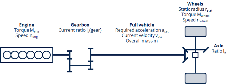
The powertrain model in Fig. 55 is used to further derive the engine speed $n_{eng}$ using the gear ratio $i_{g} (gear)$ of the currently engaged gear and axle ratio $i_{a}$ .

Fig. 55 Illustration of the powertrain model and its parameters and state variables

$n_{eng} = n_{wheel} \cdot i_{a} \cdot i_{g} (gear)$

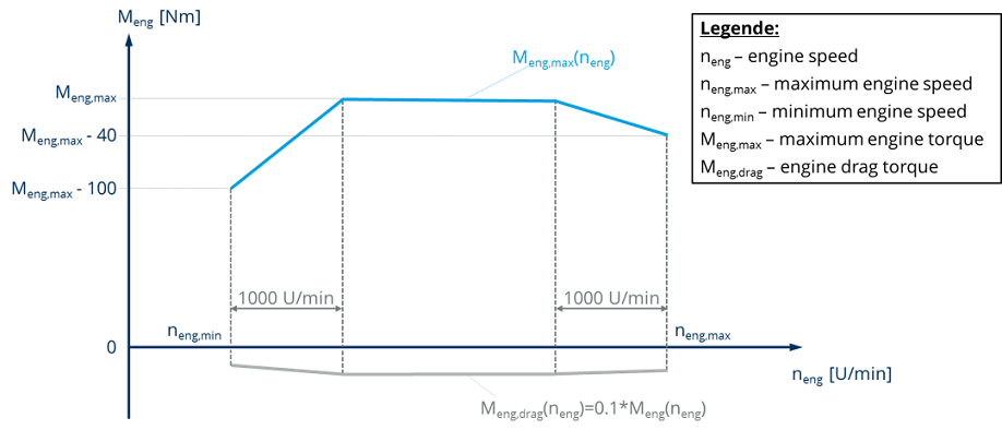
Using the engine torque map shown in Fig. 56 the maximum torque $M_{eng,max} (n_{eng})$ at the current engine speed is determined.

At this point the module differntiates between deceleration and acceleration by checking wether the value of $pos_{actuator}$ is positive or negative. Negative values stand for the use of the brake pedal between 0-100% while positive values represent the use of the accelerator pedal.

Driving resistance: First of all there are driving resistances to be considered during the drive due to the rolling resistance of tires and air resistance which could be calculated according to the follwing relations in fluid mechanics, where $\rho_{air}$ stands for air density in $km / m^3$ :

$a_{AirDrag} = - \frac{\rho_{air} \cdot c_{w} \cdot A_{proj} \cdot v_{act_{i-a}}^2}{2 \cdot m_{vehicle}}$

$a_{RollingDrag} = c_{R} \cdot 9.81 \frac{m}{s^2}$

The rolling resistance of vehicle is currently set as a dummy value (0.0125), because the related value is not in the catalog of vehicle models yet and therefore it still can not be tapped in interface.

Decelerating: When decelerating $a_{act}$ is the sum of the acceleration resulting from engine drag $a_{drag}$ and acceleration from braking $a_{actuator}$ . Whenever the driver is braking the module assumes that the engine is dragging with a moment equal to 10% of the maximum torque at the current engine speed.

$M_{drag}(n_{eng}) = - 0.1 \cdot M_{eng,max}(n_{eng})$

$M_{wheel} = \frac{M_{drag}(n_{eng})}{i_{a} \cdot i_{g}(gear)}$

$F_{wheel} = \frac{M_{wheel}}{r_{stat}}$

$a_{drag} = \frac{F_{wheel}}{m_{vehicle}}$

The maximum braking deceleration $a_{brake,max}$ is set to 9.81m/s². The actual braking power is proportional to the position of the braking pedal.

$a_{brake} = pos_{actuator} \cdot a_{brake,max}$

$a_{act} = a_{drag} + a_{brake}$

Acceleration: When the driver applies pressure on the accelerator the applied engine torque $M_{eng,act}$ is calculated as proportional to the accelerator pedal position and the span between engine drag and maximum engine torque $M_{eng}$ ( $n_{eng}$ ) at the current engine speed.

$M_{eng}(n_{eng}) = M_{drag}(n_eng) + pos_{actuator}(M_{eng,max}(n_{eng}) - M_{drag}(n_{eng}))$

$M_{wheel} = \frac{M_{eng,act}}{i_{a} \cdot i_{g}(gear)}$

$F_{wheel} = \frac{M_{eng,act}}{r_{stat}}$

$a_{act} = \frac{F_{wheel}}{m_{vehicle}}$

Once the acceleration of the vehicle is known the change in velocity is determined by its discrete time integral.

$\Delta v = a_{act} \cdot \frac{\Delta t_{cycle}}{1000}$

The sum of the previous velocity and change in velecity result in the actual vehicle velocity of the current time step:

$v_{act_{i}} = v_{act_{i-1}} + \Delta v$

Lateral dynamics

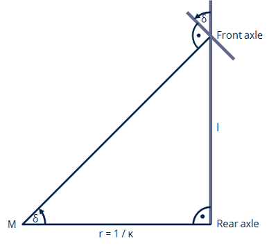
The lateral dynamics model is based on the Ackerman model which reduces the steering kinematics to a single surrogate front wheel. Considering the relatively small steering angles when driving on the highway this simplification is deemed suitable. The heading is updated using the previous heading and the change in yaw due to the steering wheel angle which is converted into a yaw rate using the simplified Ackermann model shown in Fig. 57.

Fig. 57 Illustration of the Ackermann model

Variable	Meaning	Unit	Source
$\delta_{h}$	steering wheel angle	°	AlgorithmLateralDriver
$\Phi_{act_{i-1}}$	heading at previous time step	°	WorldObjectInterface
$i_{s}$	steering ratio	/	vehicleModelParameters
$l_{wheelbase}$	wheelbase	m	vehicleModelParameters
$\Delta s$	distance travelled since last time step	m	previously calculated in the module
$\Delta t_{cycle}$	cycle time	ms	ModellInterface

The steering wheel angle $\delta_{h}$ is proportional to the front wheel angle $\delta$ :

$\delta = \frac{\delta_{h}}{i_{s}}$

The Ackermann model provides the geometric connection between the front wheel angle and the resulting curvature $\kappa$ :

$\kappa = \frac{tan(\delta)}{l_{wheelbase}}$

The combination of curvatur $\kappa$ and driven distance at that curvature $\Delta s$ result in the change of the heading $\Delta \Phi$ :

$\Delta \Phi = atan(\kappa \cdot \Delta s)$

The new heading $\Phi_{act_{i}}$ is the old heading $\Phi_{act{i-1}}$ plus the previously calculated change in heading $\Delta \Phi$ :

$\Phi_{act_{i}} = \Phi_{act_{i-1}} + \Delta \Phi$

Updating position

Once the new vehicle speed $v_{act_{i}}$ is determined the distance travelled during the last timestep $\Delta s$ is determined:

$\Delta s = v_{act_{i}} \cdot \Delta t_{cycle}$

Using the actual vehicle yaw angle in the road coordinate $\Phi_{act_{i-1}}$ the vehicles new x- and y-coordinates are calculated:

$x_{agent_{i}} = x_{agent_{i-1}} + \Delta s \cdot cos(\Phi_{act_{i-1}})$

$y_{agent_{i}} = y_{agent_{i-1}} + \Delta s \cdot sin(\Phi_{act_{i-1}})$