Algorithm_Lateral

This module is responsible for the control of the vehicle’s lateral behavior. It converts the lateral input of the driver module into a steering wheel angle. The steering wheel angle can then be forwarded to a vehicle dynamics module like Dynamics_RegularDriving.

Detailed description of the module’s features

Algorithm_Lateral receives its command variables from a driver behavior model (or an ADAS) and generates the steering wheel angle of the driver to match these command variables. The steering wheel angle parts of all controllers are summed up to the overall steering wheel angle of the driver, which is then sent to a vehicle dynamics module like Dynamics_RegularDriving. The control loop is closed by the movement of the vehicle in the world, which is again monitored by the driver behavior model. This overall control loop of vehicle lateral guidance involving Algorithm_Lateral is illustrated in the following image with the following variables:

$\kappa_{act}$ is the actual curvature of the vehicle

Four variables containing the information needed for the open-loop controller:

$\kappa_{road}$ is the curvature at the front center (i.e. center of the front of the bounding box) of the ego vehicle. It uses the vectors:
$\kappa_{segment,near}$ containing the curvatures of several segments starting at the front center up to 2m in front of the vehicles leading edge
$\kappa_{segment,far}$ containing the curvatures of several segments starting 2m in front of the vehicle and ending 8m in front of it
$\kappa_{manoeuvre}$ containing the curvature of the planned trajectory relative to the road

Other variables:

$w_{act}$ is the actual lateral position of the vehicle in the road coordinate system
$\Delta$ w is the lateral deviation
$\phi_{act}$ is the actual heading angle of the vehicle in the road coordinate system
$\Delta$ $\phi$ is the heading error
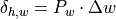
$\delta_{h,\kappa}$ is the steering wheel angle from the curvature controller
$\delta_{h,w}$ is the steering wheel angle from the lateral deviation controller
$\delta_{h,\phi}$ is the steering wheel angle from the heading error controller
$\delta_h$ is the overall steering wheel angle of the driver

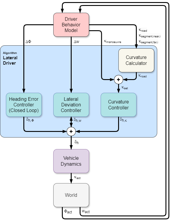
Components and signal flow of the lateral guidance control loop

The following subsections describe the theoretical background and the transfer functions of the different controllers.

Lateral dynamics

The lateral dynamics model is based on the Ackermann model which is a simple geometric expression for the relationship between the steering angle at the front wheels and the curvature the vehicle produces from it. It has several simplifications, where the most notable is the reduction of the wheels of one axle to a single surrogate wheel. This is suitable under the consideration that the steering angles of the front wheels are rather small and do not differ much between the left and the right front wheel. The first simplification may not hold up in city traffic with high curvatures. Therefore the closed-loop-controller must have increased gains in these situations. $\kappa_{road}$ , $\kappa_{segment,near}$ and $\kappa_{segment,far}$ are smoothed and weighted before adding $\kappa_{manoeuvre}$ to form $\kappa_{target}$ .

The Ackermann model is illustrated in the following image with the following variables:

$l$ is the wheelbase of the vehicle
$\delta$ is the surrogate steering angle at the front wheels towards the vehicle’s longitudinal axis
$M$ is the instantaneous centre of rotation, around which the vehicle is driving on a curve
$r$ is the radius of the curve, which the vehicle is driving around M
$\kappa$ is the curvature of this curve, which is simply the inverse of r

In accordance to the current definitions of coordinate systems, the coordinate reference point of the vehicle is considered to be the rear axle center. Therefore, the curvature of the vehicle is also expressed towards the rear axle center and not to the centre of gravity, which is why the centre of gravity is not depicted in illustration of the Ackermann model.

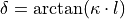
The equation derived from the Ackermann model states the following relation between the surrogate steering angle $\delta$ of the front wheels and the curvature $\kappa$ described by the rear axle around the instantaneous centre of rotation $M$ :

$\kappa = \frac{\tan(\delta)}{l}$

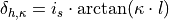
This equation can be inverted to express a required steering angle $\delta$ to adjust a specific curvature $\kappa$ :

$\delta = \arctan(\kappa \cdot l)$

To convert this into the required steering wheel angle $\delta_{h,\kappa}$ , the ratio $i_s$ of the steering gear must be applied:

$\delta_{h, \kappa} = i_{s} \cdot \arctan(\kappa \cdot l)$

The vehicle parameters $l$ and $i_s$ are received from the module Parameters_Vehicle.

Heading controller

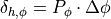
The heading controller is designed as a simple proportional controller. The general transfer function of a P-controller with the input signal heading error $\Delta\phi$ and the output signal steering wheel angle $\delta_{h,\phi}$ is described as:

$\delta_{h, \phi} = P_{\phi} \cdot \Delta\phi$

The controller amplification $P_\phi$ is therefore described as the ratio between input signal and output signal:

$P_{\phi} = \frac{\delta_{h,\phi}}{\Delta\phi}$

The controller amplification $P_\phi$ therefore expresses, how many degrees of steering wheel angle are generated by one degree heading error. The design of this controller amplification $P_\phi$ uses some considerations about plane driving kinematics of Kramer. First of all, the heading error $\Delta\phi$ is derived from the current curvature $\kappa$ of the vehicle over the change of distance $ds$ along the road’s longitudinal coordinate $s$ in one time step:

$\Delta\phi = \arctan(ds \cdot \kappa)$

Under the consideration of small angular changes in one time step, this equation can be linearized to:

$\Delta\phi = ds \cdot \kappa$

The curvature $\kappa$ of the vehicle can be substituted by an Ackermann model (see here for further information about that):

$\Delta\phi = \frac{ds \cdot \tan(\delta)}{l}$

This equation can also be linearized under the consideration of small angles:

$\Delta\phi = \frac{ds \cdot \delta} {l}$

The connection to the steering wheel angle $\delta_{h,\phi}$ can be applied by the ratio $i_s$ of the vehicle’s steering gear:

$\Delta\phi = \frac{ds \cdot \delta_{h,\phi}}{i_s \cdot l}$

This equation can be transformed to a similar form as the controller’s transfer function above:

$\frac{i_s \cdot l}{ds} = \frac{\delta_{h,\phi}}{\Delta\phi}$

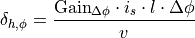
The usage of the incremental difference $ds$ in this equation is problematic, because the controller amplification becomes dependent on the simulation step size. Because of this, the absolute change $ds$ of the longitudinal road coordinate $s$ is substituted by the vehicle’s absolute velocity $v$ as a simplification, which is the change of travelled distance with respect to time:

$\frac{i_s \cdot l}{v} = \frac{\delta_{h,\phi}}{\Delta\phi}$

To tune the absolute influence of the heading controller in the overall control loop, an additional gain factor $\text{Gain}_{\Delta\phi}$ is applied to this transfer function, which allows a situation dependent amplification of the heading controller by the driver behavior model:

$\delta_{h,\phi} = \frac{\text{Gain}_{\Delta\phi} \cdot i_s \cdot l \cdot \Delta\phi}{v}$

The vehicle parameters $l$ and $i_s$ are received from the module Parameters_Vehicle, the vehicle’s absolute velocity $v$ is received from the module Sensor_Driver, and the additional controller gain $\text{Gain}_{\Delta\phi}$ is received from a driver behavior model.

Lateral deviation controller

The lateral deviation controller is designed as a simple proportional controller. The general transfer function of a P-controller with the input signal lateral deviation $\Delta$ w and the output signal steering wheel angle $\delta_{h,w}$ is described as:

$\delta_{h,w} = P_w \cdot \Delta w$

The controller amplification $P_w$ is therefore described as the ratio between input signal and output signal:

$P_w = \frac{\delta_{h,w}}{\Delta w}$

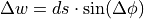
The controller amplification $P_w$ therefore expresses, how many degrees of steering wheel angle are generated by one metre of lateral deviation. The design of this controller amplification $P_w$ uses some considerations about plane driving kinematics of Kramer. First of all, the lateral deviation $\Delta$ w is derived from the current heading error $\Delta\phi$ over the change of distance $ds$ along the road’s longitudinal coordinate $s$ in one time step:

$\Delta w = ds \cdot \sin(\Delta\phi)$

The current heading error $\Delta\phi$ can further be substituted by an expression of $ds$ and the current curvature $\kappa$ of the vehicle (see Heading controller for that matter):

$\Delta w = ds \cdot \sin(\arctan(ds \cdot \kappa))$

Under the consideration of small angular changes in one time step, this equation can be linearized to:

$\Delta w = ds^2 \kappa$

The curvature $\kappa$ of the vehicle can be substituted by an Ackermann model (see here for further information about that):

$\Delta w = \frac{ds^2 \tan(\delta)}{l}$

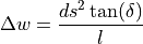
This equation can also be linearized under the consideration of small angles:

$\Delta w = \frac{ds^2 \cdot \delta}{l}$

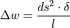
The connection to the steering wheel angle $\delta_{h,w}$ can be applied by the ratio $i_s$ of the vehicle’s steering gear:

$\Delta w = \frac{ds^2 \cdot \delta_{h,w}}{i_s \cdot l}$

This equation can be transformed to a similar form as the controller’s transfer function above:

The usage of the incremental difference $ds$ in this equation is problematic, because the controller amplification becomes dependent on the simulation step size. Because of this, the absolute change $ds$ of the longitudinal road coordinate $s$ is substituted by the vehicle’s absolute velocity $v$ as a simplification, which is the change of travelled distance with respect to time:

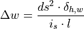
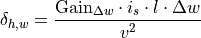
To tune the absolute influence of the lateral deviation controller in the overall control loop, an additional gain factor $\text{Gain}_{\Delta w}$ is applied to this transfer function, which allows a situation dependent amplification of the lateral deviation controller by the driver behavior model:

$\delta_{h,w} = \frac{\text{Gain}_{\Delta w} \cdot i_s \cdot l \cdot \Delta w}{v^2}$

The vehicle parameters $l$ and $i_s$ are received from the module Parameters_Vehicle, the vehicle’s absolute velocity $v$ is received from the module Sensor_Driver, and the additional controller gain $\text{Gain}_{\Delta w}$ is received from a driver behavior model.