Module 5.6: Exercises
You will now practice what you have learned in this fourth module. When modeling, there is generally not one correct answer, as multiple solutions are possible. After you complete an exercise, an example solution is given, together with an explanation.
Exercise 1
A vending machine waits to receive an order. Once a person presses on the button to start the order, it takes on average 12 second for the person to make a decision and pay. After that, a product is selected and paid, and it takes 3 seconds for the vending machine to process everything. When the vending machine is done processing, the order is retrieved in 4 seconds and the vending machine goes back to its waiting stage.
Make a model of the vending machine.
Do not use the variable time, but instead use a continuous variable to define when the automaton should go to the next location.
                                            automaton VendingMachine:
                                                event order;
                                                cont t der 1;

                                                location Idle:
                                                    initial;
                                                    marked;
                                                    edge order do t := 0.0 goto Decision;

                                                location Decision:
                                                    edge when t >= 12 do t := 0.0 goto Processing;

                                                location Processing:
                                                    edge when t >= 3 do t := 0.0 goto Retrieving;

                                                location Retrieving:
                                                    edge when t >= 4 goto Idle;
                                            end
The automaton waits for the order event to occur.
This event can come at any time.
Then, a series of activities occurs, each of which is timed.
Since we don't care about the event for these edges, we implicitly use event tau.
To be able to use relative times, we reset continuous variable t before each timed activity.
We do not reset it when we go back to Idle, as it is not necessary, since the edges in that location doesn't use t and resets it becomes necessary for the next location.
Exercise 2
Consider again the water level model that was used earlier in the module to demonstrate a timed livelock. Change the model as follows:
- Fix the livelock.
- Change the water level, such that it is between 0 and 25 meters.
- Change the rise and drop velocity of the water to 5 meters per minute, assuming the time unit of the model is in minutes.
                                            automaton WaterLevel:
                                                event rise, drop;
                                                cont level;

                                                location Rising:
                                                    initial;
                                                    marked;
                                                    equation level' = 5;
                                                    edge drop when level >= 25 goto Dropping;

                                                location Dropping:
                                                    equation level' = -5;
                                                    edge rise when level <= 0  goto Rising;
                                            end
We use two locations, one for rising and one for dropping water levels.
We use the derivative of the water's level to specify the velocity, instead of using a discrete variable.
We have edges that indicate when to go to the other location.
These edges are only enabled once the automaton should switch locations, and thus there is no timed livelock.
We opted for equations per location for the velocity of the water level rising and dropping.
This way the values are tied to the locations directly.
We could have also specified it with the declaration, using an if or switch expression.
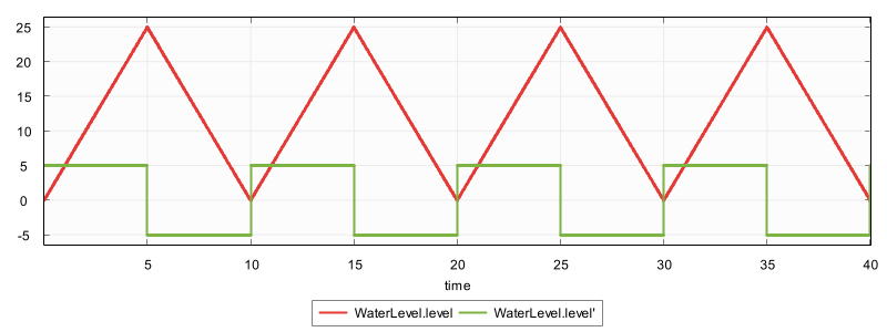
The model behaves as follows, for the first 40 time units:

Exercise 3
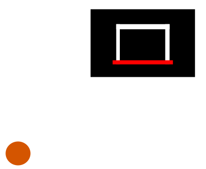
Consider a basketball (shown as a brown circle) being thrown at a backboard (shown as a large rectangle), bouncing off that backboard, and going through the hoop (also known as the ring, shown as a red line):

Some files for this exercise can be found in the course files, in the basketball folder of the module5 folder:
basketball.cif: The model of the behavior of the basketball, which is to be completed.basketball.svg: The SVG image shown above, which is used for visualization and interaction.simulation.cif: The simulation model for the basketball, which is to be completed.simulation.tooldef: The simulation script to easy start the simulation.
A player will throw the basketball against the backboard, such that it bounces off it and goes through the hoop.
A part of the basketball's behavior is already modeled in basketball.cif:
                            automaton basketball:
                                uncontrollable u_throw;

                                cont x der ...

                                cont y der ...

                                location Rest:
                                    initial;
                                    marked;
                                    edge u_throw goto Thrown;

                                location Thrown:
                                    edge ...
                            end
Initially the basketball is in Rest at the position shown in the image above.
The basketball can be thrown by the player with the u_throw event.
It is then thrown and flies linearly through the air towards the backboard.
The basketball's position is modeled by its x and y coordinates.
Once the ball goes through the hoop, the simulation automatically resets back to its resting state.
You need to adapt the parts indicated by ... to complete the model.
In simulation.cif, the visualization and interaction is defined:
                            import "basketball.cif";
                            svgfile "basketball.svg";

                            const real SCALE_FACTOR = 10;

                            svgin id "basketball" event basketball.u_throw;

                            svgout id "basketball" attr "transform"
                                value fmt("translate(%s, -%s)", ... * SCALE_FACTOR, ... * SCALE_FACTOR);
The u_throw is coupled to a click on the basketball.
The position of the basketball is partially defined by the SVG output mapping.
You need to still fill in the ... parts.
The basketball.cif file can be adapted as follows:
                                            automaton basketball:
                                                uncontrollable u_throw;

                                                cont x der switch self:
                                                               case Rest:    0.0
                                                               case Thrown:  2.5
                                                               case Bounced: 3.5
                                                           end;

                                                cont y der switch self:
                                                               case Rest:     0.0
                                                               case Thrown:   3.0
                                                               case Bounced: -3.0
                                                           end;

                                                location Rest:
                                                    initial;
                                                    marked;
                                                    edge u_throw goto Thrown;

                                                location Thrown:
                                                    edge when y >= 6 goto Bounced;

                                                location Bounced:
                                                    edge when x >= 8 do x := 0, y := 0 goto Rest;
                                            end
The simulation.cif file can be adapted as follows:
                                            import "basketball.cif";
                                            svgfile "basketball.svg";

                                            const real SCALE_FACTOR = 10;

                                            svgin id "basketball" event basketball.u_throw;

                                            svgout id "basketball" attr "transform"
                                                value fmt("translate(%s, -%s)", basketball.x * SCALE_FACTOR, basketball.y * SCALE_FACTOR);
We set the derivatives such that the linear movement after throwing goes to the blackboard, and the linear movement after bouncing goes through the hoop. We use two separate locations for them, to allow having different derivatives for the two movements. For the simulation model, we simply fill in the coordinates of the basketball.
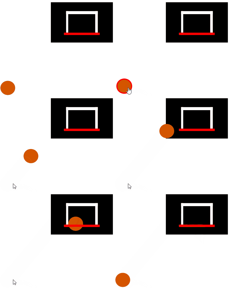
The simulation then looks something like this:

Exercise 4
Consider again the phone model from earlier in the module. You will now make a more realistic model of a phone, that allows using and charging the phone as long as you want, and even simultaneously.
An SVG image file named phone.svg can be found in the course files, in the phone folder of the module5 folder:

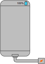
The rectangle with rounded borders represents the phone. At its top right is the battery indicator, both as a light-blue bar and as a text. At the bottom is its power connector. The power connector is connected to the charging cable. The charging cable is connected to the charger, the bottom-right box with the charging icon.
a. Model the behavior of the phone that can be used and charged.
Model the phone's behavior in phone.cif, taking into account the following:
- Use two events for toggling usage of the phone and the charger being connected.
- Track the usage of the phone and the charger being connected using discrete variables.
- The phone is initially fully charged, not being used and the charging cable is disconnected.
- The phone charges with 8% per time unit, while using the phone requires 5% of the battery's capacity per time unit.
- If the battery has no charge left, the phone can't be used.
- The battery can't be less than empty or more than 100% charged.
The phone.cif file could look like this:
                                            automaton phone:
                                                uncontrollable u_usage_toggle;
                                                uncontrollable u_charger_connected_toggle;

                                                disc bool is_using = false;
                                                disc bool is_connected = false;

                                                alg real charge_increase = if is_connected: 8 else 0 end;
                                                alg real usage_decrease  = if is_using:     5 else 0 end;
                                                alg real total_increase  = charge_increase - usage_decrease;
                                                alg real battery_delta   =
                                                            if   battery_percentage <= 0   and total_increase < 0: 0
                                                            elif battery_percentage >= 100 and total_increase > 0: 0
                                                            else                                                   total_increase
                                                            end;

                                                cont battery_percentage = 100 der battery_delta;

                                                location:
                                                    initial;
                                                    edge u_usage_toggle when battery_percentage > 0 do is_using := not is_using;
                                                    edge when battery_percentage <= 0 and is_using do is_using := false;
                                                    edge u_charger_connected_toggle do is_connected := not is_connected;
                                            end
The phone has a u_usage_toggle event to toggle using the phone.
It also has a u_charger_connected_toggle event to toggle the charger being connected to the phone.
The events are uncontrollable as the user decides when they want to use the phone or when the connect or disconnect the charging cable.
The is_using variable tracks usage of the phone, while the is_connected variable tracks whether the charging cable is connected.
Initially, the phone is not being used and the charging cable is disconnected, so both variables are initially false.
We then define various algebraic variables.
Variable charge_increase indicates the increase of the battery percentage per unit, due to the charging cable being connected.
If the charging cable is connected, the increase is 8 percent per unit.
If the charging cable is disconnected, the battery percentage does not increase.
Similarly, usage_decrease indicates whether the battery percentage decreases per time unit, and how much.
The total_increase variable accounts for both usage and charging, which may be active at the same time.
Finally, battery_delta accounts for the fact that the battery percentage must at all times remain between 0 and 100 percent.
That is, we can't be more empty than fully empty, and we can't charge an already fully charged phone.
The current battery percentage is tracked in the battery_percentage continuous variable.
Initially, the phone is fully charged, so the battery percentage is 100 percent.
The derivative is defined to be battery_delta.
There is a single location with three edges.
The first edge handles the u_usage_toggle event.
It flips the is_using variable.
However, you can use the phone when the battery is fully drained, so then the phone can't be used.
We thereby also disallow to stop using the phone when the battery is fully drained, but this is OK, because that is already handled by the second edge.
The second edge ensures that if the phone's battery is fully drained, we stop using the phone, even if the user doesn't want to.
This edge uses a tau event, which is not influenced by anything the user can do.
The third edge handles the u_charger_connected_toggle event.
It flips the is_connected boolean.
b. Create a simulation model for the phone.
Model the phone's behavior in simulation.cif, taking into account the following:
- Connect the event to toggle the charger being connected to the charger, which has id
charger. - Connect the event to toggle the usage of the phone to the phone's screen, which has id
phone-screen. -
Ensure the battery percentage text is correctly updated based on the state of the phone.
The battery percentage text element has id
battery-percentage. -
Ensure the battery level (light-blue bar) correctly displays the battery status.
The rectangle has id
battery-level. If the phone is fully charged, the height of this rectangle should be3.16. - Ensure that the phone's screen is
whiteis the phone is being used, and isblackotherwise. -
Ensure that the charger cable is visible when it is connected, and is invisible otherwise.
The charger cable has id
charger-cable. Hint: Use thedisplayattribute, with valueinheritto show the element andnoneto hide the element.
Hint: Note that negative heights are invalid in SVG, so you may need to cap certain values.
The simulation.cif file could look like this:
                                            import "phone.cif";
                                            svgfile "phone.svg";

                                            svgin id "charger"      event phone.u_charger_connected_toggle;
                                            svgin id "phone-screen" event phone.u_usage_toggle;

                                            svgout id "battery-percentage" text value fmt("%.0f%%", capped_percentage);
                                            svgout id "battery-level" attr "height" value scale(capped_percentage, 0, 100, 0, 3.16);
                                            svgout id "phone-screen" attr "fill" value if phone.is_using: "white" else "black" end;
                                            svgout id "charger-cable" attr "display" value if phone.is_connected: "inherit" else "none" end;

                                            alg real capped_percentage = min(max(phone.battery_percentage, 0), 100);
We import the phone's behavior from phone.cif.
We connect the simulation model to the phone.svg image.
We connect the interactive events to the interactive elements of the image using two SVG input mappings.
There are four SVG output mappings, one for each element that requires visualization.
The battery percentage text is set using an SVG output mapping that sets the text based on a format pattern.
The %.0f part of the pattern formats the value as a floating point number with zero digits after the decimal, so as whole numbers.
The %% part of the pattern inserts an escaped percentage character.
The battery level bar is set by scaling the percentage, which is in the range 0 to 100, to the height of the bar, which is 0 to 3.16. The phone's screen is set to the right color, and the charger cable is shown or hidden.
To prevent a negative height for the battery level bar's rectangle, we cap the battery percentage of the phone to be at least zero.
We also cap it to be at most 100, to prevent a too high bar.
We therefore define capped_percentage, which is minimally 0, by taking the maximum of the battery percentage and 0.
It is also maximally 100, by taking the minimum of the bottom-capped percentage and 100.
We use this bottom-and-top-capped percentage for both the height of the phone's bar rectangle, and for the battery percentage text.
This also prevents displaying percentage texts that are less than zero or higher than 100.
C. Simulate the phone's behavior, and check that it is correct.
Create a ToolDef script to simulate the phone's behavior and interact with it via the SVG image. Try various scenarios, such as combinations of the phone being in use or not in use, and the charging cable being connected and disconnected. Also, check what happens when the phone gets fully depleted, or becomes fully charged.
The simulation.tooldef file could look like this:
                                            from "lib:cif" import *;

                                            cifsim(
                                                "simulation.cif",
                                                "--input-mode=svg",
                                                "--auto-algo=first",
                                                "--frame-rate=60",
                                                "--option-dialog=no",
                                            );
The model should work as expected.
Exercise 5
Consider again the elevator model from Exercise 3 and Exercise 7 of the previous module.
The final model after Exercise 7 of the previous module is provided in the course files, in the elevator folder of the module5 folder.
This is the model with the building that has three floors, the elevator, a sensor at each floor to detect whether the elevator is at that floor, and a button at each floor to request the elevator to move to that floor.
The state of the plant is visualized, and the button are connected to events.
We continue with this model, adding timing for the movement of the elevator, and synthesizing a supervisor to control it based on the floor requests.
a. Separate the plants and requirements from the simulation model.
The current model contains the plant, as well as connections to the SVG image for simulation. We want to add timing for the simulation, but timed models are not supported for synthesis. Therefore, separate the plant model from the simulation model. Make sure to still have a scalable simulation model.
The elevator.cif file with the plant model could look like this:
                                            plant def Sensor(alg bool initialOn; alg bool isOn):
                                                uncontrollable u_on, u_off;

                                                location Off:
                                                    initial not initialOn;
                                                    marked not initialOn;
                                                    edge u_on  when     isOn goto On;

                                                location On:
                                                    initial initialOn;
                                                    marked initialOn;
                                                    edge u_off when not isOn goto Off;
                                            end

                                            sensor_top:    Sensor(false, elevator.floorNr = 3);
                                            sensor_middle: Sensor(false, elevator.floorNr = 2);
                                            sensor_bottom: Sensor(true,  elevator.floorNr = 1);

                                            plant def Button():
                                                uncontrollable u_pushed, u_released;

                                                location Released:
                                                    initial;
                                                    marked;
                                                    edge u_pushed goto Pushed;

                                                location Pushed:
                                                    edge u_released goto Released;
                                            end

                                            button_top:    Button();
                                            button_middle: Button();
                                            button_bottom: Button();

                                            plant def Observer(event request; alg bool atFloor):
                                                uncontrollable u_reset;

                                                location NotRequested:
                                                    initial;
                                                    marked;
                                                    edge request goto Requested;

                                                location Requested:
                                                    edge u_reset when atFloor goto NotRequested;

                                            end

                                            observer_top:    Observer(button_top.u_pushed,    sensor_top.On);
                                            observer_middle: Observer(button_middle.u_pushed, sensor_middle.On);
                                            observer_bottom: Observer(button_bottom.u_pushed, sensor_bottom.On);

                                            plant elevator:
                                                controllable c_up, c_down;
                                                disc int[1..3] floorNr = 1;

                                                location:
                                                    initial;
                                                    marked;
                                                    edge c_up   when floorNr < 3 do floorNr := floorNr + 1;
                                                    edge c_down when floorNr > 1 do floorNr := floorNr - 1;
                                            end
The SVG file declaration has been removed, as well as the SVG input and output mappings. The no longer needed algebraic parameters of the automaton definitions are also removed. And the automaton instantiations have been updated to no longer provide arguments for these removed parameters.
The simulation.cif file with the SVG image connections could look like this:
                                            import "elevator.cif";
                                            svgfile "elevator-with-buttons.svg";

                                            group def SensorSim(alg bool sensorOn; alg string floorName):
                                                svgout id "sensor-" + floorName attr "display" value if sensorOn: "inherit" else "none" end;
                                            end

                                            sensor_sim_top:    SensorSim(sensor_top.On,    "top");
                                            sensor_sim_middle: SensorSim(sensor_middle.On, "middle");
                                            sensor_sim_bottom: SensorSim(sensor_bottom.On, "bottom");

                                            group def ObserverSim(alg bool observerNotRequested; alg string floorName; event request):
                                                svgout id "button-" + floorName attr "fill" value if observerNotRequested: "red" else "limegreen" end;
                                                svgin id "button-" + floorName event request;
                                            end

                                            observer_sim_top:    ObserverSim(observer_top.NotRequested,    "top",    button_top.u_pushed);
                                            observer_sim_middle: ObserverSim(observer_middle.NotRequested, "middle", button_middle.u_pushed);
                                            observer_sim_bottom: ObserverSim(observer_bottom.NotRequested, "bottom", button_bottom.u_pushed);

                                            group elevator_sim:
                                                svgout id "elevator" attr "y" value (((3 - elevator.floorNr) * 50) + 10);
                                            end
The simulation model is imported, and the SVG file declaration is moved to the simulation model. For the sensors and observers, group definitions are included. They are group definitions, as they only contain the SVG input/output mappings, not any behavior.
The SensorSim definition for sensor simulation gets the relevant information as parameters.
It makes sure the floor sensor is correctly shown or hidden.
This SVG output mapping is nearly the same as the one we removed from the plant model, except that the 'sensor is on' status is accessed via the sensorOn parameter.
The three instantiations use names similar to the instantiations of the sensors, but with sim in them, to avoid having multiple components with the same name.
The observer definitions and instantiations are similar. By using group definitions and instantiations, we ensure there is still reuse, even though the SVG input and output mappings are now defined separately from the plant behavior.
The elevator is also put in a group, to have it be similar to the sensor and observer simulation groups.
It contains the single SVG output mapping that positions the elevator on the right floor.
It is nearly the same as the one we removed from the plant model, except that the floor number is now accessed from the elevator.
b. Add timing to the movement of the elevator.
Adapt the plant model to account for the up and down movements taking time. Adapt the simulation model to make sure that it takes two time units for the elevator to move to a different floor.
The elevator plant automaton is adapted as follows:
                                            plant elevator:
                                                controllable c_up, c_down;
                                                uncontrollable u_arrived;
                                                disc int[1..3] floorNr = 1;

                                                location Idle:
                                                    initial;
                                                    marked;
                                                    edge c_up   when floorNr < 3 and any_sensor_on goto GoingUp;
                                                    edge c_down when floorNr > 1 and any_sensor_on goto GoingDown;

                                                location GoingUp:
                                                    edge u_arrived do floorNr := floorNr + 1 goto Idle;

                                                location GoingDown:
                                                    edge u_arrived do floorNr := floorNr - 1 goto Idle;
                                            end
The c_up and c_down events no longer immediately lead to reaching a different floor.
Instead, they lead to a different location, where the elevator is going up or down.
A new uncontrollable event u_arrived indicates that the next floor is reached.
The event is uncontrollable as the controller can't prevent reaching the floor once the movement has commenced.
And we must specify the controllability of the event in the plant model, as synthesis requires it.
Once the elevator arrives at the next floor, the floorNr is updated, and the elevator is Idle again.
The up and down movements are only allowed once any sensor is on.
This prevents moving between floors and never turning on the sensor for that floor.
This is important to make sure that the observers can be reset.
We thus introduce this any_sensor_on variable, while also adapting the sensors themselves:
                                            sensor_top:    Sensor(false, elevator.floorNr = 3 and elevator.Idle);
                                            sensor_middle: Sensor(false, elevator.floorNr = 2 and elevator.Idle);
                                            sensor_bottom: Sensor(true,  elevator.floorNr = 1 and elevator.Idle);

                                            alg bool any_sensor_on = sensor_top.On or sensor_middle.On or sensor_bottom.On;
Algebraic variable any_sensor_on is true if any of the sensors is on.
We also add a and elevator.Idle condition for sensors to go on, since the floor is now only updated after having completed a move.
This takes time, and during that time, the floor number still indicates the old floor.
The sensor must however go off as soon as the elevator leaves the floor.
The elevator_sim group in the simulation model is adapted as follows:
                                            automaton elevator_sim:
                                                cont t der 1;

                                                location Idle:
                                                    initial;
                                                    edge elevator.c_up, elevator.c_down do t := 0 goto Moving;

                                                location Moving:
                                                    edge elevator.u_arrived when t >= 2 goto Idle;

                                                svgout id "elevator" attr "y" value (((3 - elevator.floorNr) * 50) + 10);
                                            end
The group is changed to an automaton, to allow adding behavior to it.
There is a continuous variable t to track time passage.
There are two locations, Idle and Moving.
There is no need to have separate locations for going up and down, as the time for both is the same.
If we either go up or down, we set t to 0 to start measuring time from that moment forward, and we go to the Moving location.
There we wait for two time units, before we enable the u_arrived event.
This way, the plant automaton elevator gets restricted and has to wait as well, as they both synchronize over the u_arrived event.
Once the elevator arrived, it goes back to being Idle again.
c. Adapt the visualization to make the elevator move continuously between floor.
The elevator_sim automaton in simulator.cif could be adapted as follows:
                                            automaton elevator_sim:
                                                cont t der 1;

                                                const real duration = 2;

                                                alg real simFloorNr = elevator.floorNr + switch elevator:
                                                                                             case Idle:        0
                                                                                             case GoingUp:     t / duration
                                                                                             case GoingDown: -(t / duration)
                                                                                         end;

                                                location Idle:
                                                    initial;
                                                    edge elevator.c_up, elevator.c_down do t := 0 goto Moving;

                                                location Moving:
                                                    edge elevator.u_arrived when t >= duration goto Idle;

                                                svgout id "elevator" attr "y" value (((3 - simFloorNr) * 50) + 10);
                                            end
Instead of using elevator.floorNr, the SVG output mapping now uses simFloorNr.
The new simFloorNr algebraic variable adds to the elevator.floorNr the partial movement to another floor.
If the elevator is Idle, there is no partial movement.
Otherwise, it is the timer value t, divided by two, as in two time units it moves one floor.
The value is positive or negative, depending on the direction in which the elevator is moving.
We opt to put the value 2 in a constant, to be able to more easily adapt it.
d. Add requirements to ensure that the elevator only moves when requested, and goes to the right floor.
Add the requirement to the plant model. Synthesize a supervisor from the plants and requirements. Adapt the simulation model use the synthesized controlled system, rather than the plant and requirements model. Check that the elevator works as expected.
The elevator.cif model is extended with requirements:
                                            requirement elevator.c_up
                                                needs (elevator.floorNr = 1 and (observer_top.Requested or observer_middle.Requested))
                                                   or (elevator.floorNr = 2 and  observer_top.Requested);

                                            requirement elevator.c_down
                                                needs (elevator.floorNr = 3 and (observer_bottom.Requested or observer_middle.Requested))
                                                   or (elevator.floorNr = 2 and  observer_bottom.Requested);
The elevator may go from floor the bottom floor if either the top or middle floor requests the elevator. It may also go up from the middle floor if the top floor requests the elevator. Going down is similarly constrained.
The simulation.cif model gets its import statement replaced:
import "elevator.ctrlsys.cif";
It imports the result of synthesis, the controlled system model, rather than the model with plants and requirements.
Simulating the simulation model, you can see that the elevator only moves if requested. And it only goes to floors to which is requested.