Discrete, continuous, and constant distributions
CIF features over a dozen different stochastic distributions. These distributions can be categorized into three categories: discrete, continuous, and constant distributions. Discrete distributions can result in only a limited number of possible values. Examples include tossing a coin (heads and tails) and throwing a dice (six possible outcomes). Continuous distributions can result in all values from a certain range. Examples include the time it takes for a machine to produce a single product (positive amount of time), and the purity of produced medicine (0% to 100%). Constant distributions are discrete distributions that always result in the same sampled value. They are useful during the development of a model, or for debugging. The remainder of this lesson further explains these three categories, and illustrates them using some examples.
Discrete distributions
Discrete distributions can result in only a limited number of possible values. The lesson that introduced stochastics used the discrete Bernoulli distribution to model tossing of a coin, which can result in either heads or tails.
Throwing a dice can result in six possible outcomes: 1, 2, 3, 4, 5, and 6. For a fair dice, each of the outcomes is equally likely, with chance 1/6. This can be modeled using a discrete uniform distribution:
automaton dice:
  disc dist int d = uniform(1, 7);
  disc int result;
  disc list int results = [];

  location throw:
    initial;
    edge do (result, d) := sample d goto add;

  location add:
    edge do results := results + [result] goto throw;
end
The uniform function is used to create a uniform integer distribution that produces integer samples from the range [1..7) (inclusive on the left side, exclusive on the right side). Each sample is stored in result and added to the results. If we were to simulate this model forever, the results list would contain equal amounts of each of the six values.
Continuous distributions
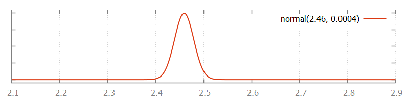
Continuous distributions return a value from a continuous range. An example is the weight of pennies. This could for instance be approximated using a continuous normal distribution with a mean of 2.46 grams and a variance of 0.0004 grams:
automaton pennies:
  disc dist int d = normal(2.46, 0.0004);

  location:
    initial;
    edge do (weight, d) := sample d;
end
The normal function is used to create a normal distribution with a mean of 2.46 and a variance of 0.0004. The sampled weight is stored in the weight variable each time the distribution is sampled. The probability of the different weights as a result of the used normal distribution is depicted in the following figure:
Constant distributions
When developing a model with stochastic behavior, it can be hard to validate whether the model behaves correctly, since the stochastic results make it difficult to predict the outcome of experiments. As a result, errors in the model may not be noticed, as they hide in the noise of the stochastic results. One solution is to first make a model without stochastic behavior, validate that model, and then extend the model with stochastic sampling. Extending the model with stochastic behavior is however an invasive change that may introduce new errors. These errors can again be hard to find due to the difficulties to predict the outcome of an experiment. The constant distributions aim to narrow the gap by reducing the amount of changes that need to be done after validation.
With constant distributions, a stochastic model with sampling of distributions is developed, but the stochastic behavior is eliminated by temporarily using constant distributions. The model performs stochastic sampling of values, but with predictable outcome, and thus with predictable experimental results, making validation easier. After validating the model, the constant distributions are replaced with the distributions that fit the mean value and variation pattern of the modeled system, giving a model with stochastic behavior. Changing the used distributions is however much less invasive, making it less likely to introduce new errors at this stage in the development of the model.
Constant distributions always produce the same sampled value. Consider the following CIF specification:
automaton dice:
  disc dist int d = constant(3); // Constant distribution.
  disc int result;
  disc list int results = [];

  location throw:
    initial;
    edge do (result, d) := sample d goto add;

  location add:
    edge do results := results + [result] goto throw;
end
This model is identical to the dice model one used earlier in this lesson, except for distribution variable d, which now holds a constant distribution that only produces value 3 when sampled.