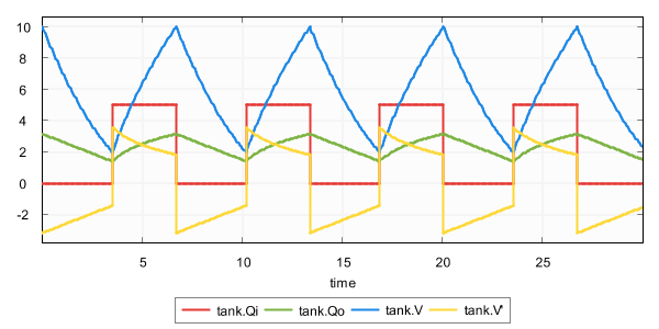
Plot visualizer
For models with variables, especially continuous ones, it may be useful to be able to observe how their values change, as time progresses during simulation. The plot visualizer can be used for that exact purpose. The plot visualizer can create graphical plots, where the x-axis represents the values of variable time, and the y-axis represents values of the variables being plotted. Here is an example screenshot of the visualizer:
Plot visualization is disabled by default. It can be enabled using the Plot visualization option (Output: Plot visualization category).
Variables
The plot visualizer can plot the values of the following variables (officially 'state objects'):
-
The state variables, which includes the discrete variables, input variables and the continuous variables.
-
The derivatives of the continuous variables. This does not include the derivative of variable
time. -
The algebraic variables.
Only variables of type bool, int (with or without ranges), or real can be plotted. For variables with a boolean type, value false is represented by 0, and value true is represented by 1.
Filtering
By default, if plot visualization is enabled, all variables (officially 'state objects') that can be plotted are plotted. The one exception is variable time, which is excluded by default, as it already represents the x-axis. That is, variables are plotted against time. Using the Plot visualization filters option (Output: Plot visualization category), the state objects can be filtered. The Plot visualization filters option only has effect if plot visualization is enabled, using the Plot visualization option.
As value for the option, comma separated filters should be supplied. Each filter specifies one or more state objects. The absolute names of the objects are used. That is, for an automaton a, with a variable x, the absolute name of the variable object is a.x. If CIF textual syntax keyword are used as names for events (such as plant), then they must be escaped in .cif files ($plant). For filters however, all escape characters ($) in the names are ignored. The * character can be used as wildcard, to indicate zero or more characters. If a filter doesn’t match any of the state objects of the CIF model, a warning is printed to the console. A warning is also printed if the entire state is filtered out.
By default, filters include matching state objects. Filters may however be preceded by a - character, turning them into exclusion filters, which exclude matching states objects rather than including them. Filters are processed in the order they are specified, allowing for alternating additions and removals. If a filter does not result in the addition/removal of any state objects to/from the filter result, a warning is printed to the console.
As an example, option value a.*,-a.b*,a.bc* consists of three filters: a.*, -a.b*, and a.bc*. The first filter indicates that state objects whose absolute names start with a. are to be included. The second filter indicates that from those matching state objects, the state objects whose absolute names start with a.b* are to be excluded. To that result, the third filter adds those state objects whose absolute names start with a.bc*. For instance, if a specification contains state objects time, a.a, a.b a.bb, a.bc, a.b.c, a.bc, a.bcc, and a.bcd, the result of the three filters is that the following state objects are displayed: a.a, a.bc, a.bc, a.bcc, and a.bcd.
The default option value (filter) is *,-time.
Multiple plot visualizers
By default, only one visualizer is shown. However, using the Plot visualization filters option (Output: Plot visualization category), it is possible to specify that multiple visualizers should be used. The option allows for filtering of the state objects, as described above. However, such filters can be separated by semicolons, to specify the filters per visualizer.
As an example, consider option value time,a.x;b.y. This results in two plot visualizers. The first one displays state objects time and a.x, while the second one displays state object b.y.
Plot visualization modes
There are two plot visualization modes:
-
Live plotting. In this mode, the plots are shown at the start of the simulation, and are continuously updated as new data becomes available during simulation.
-
Postponed plotting. In this mode, the plots are shown after the simulation has ended.
Which plot visualization mode to use, can be configured using the Plot visualization mode option (Output: Plot visualization category). Using that option it is possible to explicitly choose one of the modes. By default, an automatic mode is used, which chooses between live and postponed mode, as follows:
| Input mode vs real-time simulation | Real-time enabled | Real-time disabled |
|---|---|---|
|
Interactive console input mode (pure interactive) |
live |
live |
|
live |
postponed |
|
|
Interactive GUI input mode (pure interactive) |
live |
live |
|
live |
postponed |
|
|
live |
postponed |
|
|
live |
postponed |
|
|
live |
postponed |
When doing a non real-time simulation, using a non-interactive input mode leads to as fast as possible simulation, where a lot of data points are calculated in a short amount of time. If live plotting mode is then enabled, this floods the visualizer with so much data that it can’t keep up. The effect is a non-responsive user interface. While the automatic default can thus be overridden using the option, it is generally not recommended.
Plot visualization range
For simulations that span longer periods of (model) time, there may be too much data to display, for the limited width of the time axis (x-axis). To keep the plot useful, the range of time values to display on the x-axis can be configured using the Plot visualization range option (Output: Plot visualization category).
By default, only the 50 most recent time units are displayed. That is, if the current model time is 120, then the plot only shows the values of the variables from time 70 to time 120. Using the option, the length of the range can configured to any other positive value. The option can also be used to set the range to infinite, to display the values of the variables during the entire simulation, from time 0 to the current model time.
For long running simulations, with lots variables, using an infinite range can lead to large numbers of data points, which can have a significant effect on performance. This applies especially for live plotting mode.
Data points
This section describes which data points are visualized. For most users, this will be of little interest, as it essentially works as you would expect.
The plot visualizer adds data points (a time value and a value of a variable at that time) for all variables, for the following states:
-
The initial state of the simulation.
-
The start state of every time transition.
-
Intermediate states of time transitions, only if real-time simulation is enabled.
-
Trajectory data points of time transitions, only if real-time simulation is disabled.
-
The end state of every time transition.
For real-time simulation, the amount of model time between two intermediate states is the model time delta, and can be influenced using the frame rate and simulation speed.
For non real-time simulation, the trajectory data points are determined by the ODE solver integrator, and can be influenced using the integration options, as well as the fixed output step size option.
Relation to trajectory data output
The plot visualizer can be used for simple plotting. It can be customized a bit through options, as described above. However, the level of customization is somewhat limited. For instance, the appearance can not be customized. This is intentional.
If further customization is required, use the trajectory data output component instead. It allows saving the data to a file, for further processing with external tools, such as R.
Such post processing is then performed after the simulation has ended. A benefit of the plot visualizer, is that it allows live plotting mode, without the need of post processing, and which can be enabled with little effort. The plot visualizer is meant to be used only to get a basic understanding of how values of variables change as time progresses.
Saving a plot image
The plot visualizer can export the currently visible plot to several different image formats. To export the image, first make sure that the plot visualizer has the focus. Then select to open the Save plot as dialog. Alternatively, right click the plot itself, and choose Save As… from the popup menu, to open the Save plot as dialog. In the dialog, specify the file name of the exported image. Click OK to confirm and continue.
A second dialog appears, in which the size of the exported image can be specified. By default, the current size of the visualizer is used. A custom size can be entered. The width and height need to specified in pixels, separated by a x character. For instance, for a width of 640 pixels and a height of 480 pixels, enter 640x480 into the dialog. Click OK to confirm and to actually export the image.
The following raster image formats are supported:
-
Portable Network Graphics (
*.png) -
JPEG (
*.jpg) -
Graphics Interchange Format (
*.gif)
The image format that is used to export the image, is derived from the file extension that is used. For each of the supported file formats, the allowed file names (with file extensions) are indicated above (between parentheses).
After the image is exported, the workspace is refreshed to show that new image file, if the image was saved in a project that is visible in the Project Explorer tab or Package Explorer tab.
In order for the export to succeed, data points must be available for at least two time values.
Undo/reset
It is possible to go back in time, by undoing one or more transitions, or by resetting the simulation.
If one or more transitions are undone, data for all time points that are then suddenly in the future, are removed. More precisely, all data for time points added for time transitions that have been undone, are removed.
If the simulation is reset, the entire plot is cleared.