The basics of numeric integration
During time transitions, the values of the continuous variables and their derivatives change. The derivatives have explicit equations, the continuous variables change according to the value of their derivatives. Using the equations for the derivatives as a system of ordinary differential equations (ODEs), together with the initial values of the continuous variables as the initial conditions, this essentially comes down to solving an initial value problem (IVP).
Such problems can be solved through integration. For some problems it is possible to do this symbolically. For more complex systems of ODEs however, numerical methods are used. The CIF simulator uses The Apache Commons Mathematics Library, which contains several numerical integrators.
Linear ODE
Consider the following CIF specification, with a linear ODE:
cont x = 0.0;
equation x' = 1.0;
The solution to this IVP, is the values of continuous variable x and its derivative x', as function of variable time:
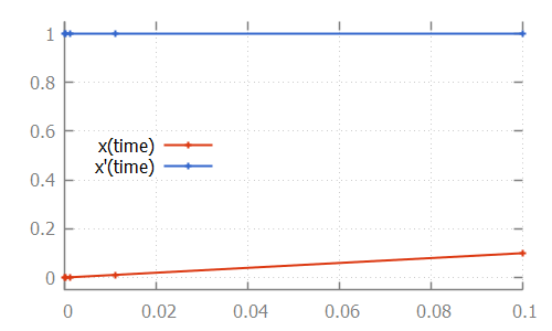
Here, the numerical integrator start with the initial value of continuous variable x, which is 0.0. For the initial value of variable time, which is also 0.0, it computes x', which is 1.0. It then slightly increases the value of variable time to say 1e-6. Assuming a linear continuous variable x, the value of variable x at that time is 1e-6 as well.
The numerical integrator tries to predict the values of the derivative as time progresses. It gradually increases the value of variable time, predicting the value of the derivative at the next time point. If the next prediction closely matches the actual calculated value, the integrator moves on to the next time point. If the next prediction is not close enough to the actual calculated value of the derivative for that time point, more intermediate values are calculated. That is, the integrator tries to approximate the derivative as time progresses, while increasing the time between two consecutive time points. As long as the predictions match the actual calculated value of the derivative at the next time point, it keeps increasing the step size even further. If the predictions are not good enough (the difference with the actual calculated value is above a certain tolerance), more intermediate time points are investigated. The values calculated for those time points can then be used to come up with a better approximation, that better predicts the value of the derivative at future time points.
For the linear ODE given above, the trajectory data calculated by the integrator is:
# time                 x                       x'
0.0                    0.0                     1.0
9.999999999999999e-5   1.0000000000000003e-4   1.0
0.0011                 0.0011000000000000005   1.0
0.0111                 0.011100000000000006    1.0
0.1                    0.10000000000000006     1.0
Note that the time points for which the values were calculated, are indicated in the figure above by small plus signs (+).
Nonlinear ODE
The approximations of the integrator don’t need to be linear. Some integrators for instance support nonlinear differential equations. Consider the following CIF specification, with such a nonlinear ODE:
The solution calculated by the numerical integrator is:
cont x = 0.0;
equation x' = (x * x) - x - 2;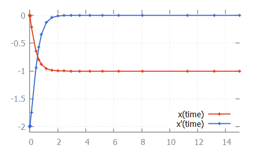
Here, we see how the step size is increased initially, as the linear approximation is good enough. As soon as we get to the bend, the step size is reduced to better approximate the actual values. After the bend, the step size is slowly increased again. The integrator internally uses a polynomial of a higher degree to approximate this differential equation.
Discontinuities
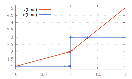
If the derivative has a discontinuity, such as in the following CIF specification:
cont x = 1.0;
equation x' = if x < 2: 1.0
              else      3.0
              end;
The integrator will try to figure out the time point at which the discontinuity occurs, by decreasing the step size as it nears the discontinuity. After the discontinuity, the step size is gradually increased, as integration continues: