The basics of numeric root finding
During time transitions, the values of the continuous variables and their derivatives change. If continuous variables or their derivatives are (directly or indirectly) used in guards of edges, changes in their values may result in the guard becoming enabled, as time progresses. To detect such changes during integration, a root finding algorithm can be used.
Consider the following CIF specification:
automaton p:
cont x = 0.0;
equation x' = 0.5;
location:
initial;
edge when x >= 1.5 do x := 0.0;
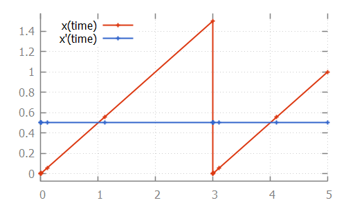
endHere, the value of continuous variable x increases with 0.5 every time unit. Once the value of 1.5 is reached, the variable is reset to 0.0. This process is repeated:
If we look at the data calculated by the numerical integrator, to solve the ODE problem:
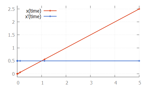
we see that values are calculated for time points 1.1111 and 5.0. If we then also look at the value of the guard, where we use value -1 for false and +1 for true:
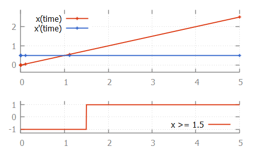
we see that at time 1.1111, the value of the guard is -1 (false). At time 5.0 it is +1 (true). That is, the guard changed value between two time points calculated by the integrator. If this is the case, the ODE solver tries to calculate the exact time point at which the guard changes its value. That is, it calculates the exact time point at which the guard function crosses the time axis, and thus has a root.
One of the simplest root finding algorithms, is the bisection method. This algorithm starts with the two time points where the guard has opposite signs. This is the interval where the guard sign change occurs (it contains the root). The bisection method tries to reduce the size of the interval, by calculating the value of the guard in the middle of the interval. Depending on the sign of the value of the guard at this middle point, this middle point replaces either the lower bound or the upper bound of the interval. This is done in such a way that the values of the guard at the lower and upper bound of the interval have opposite signs, and the interval thus brackets the root.
For the example above, the root is calculated as follows:
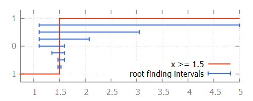
We start with the interval [1.1111 .. 5.0]. The middle point is 3.0555 at which the guard holds, just like the upper bound (at 5.0). Thus 5.0 is replaced by 3.0555. The middle point of 1.1111 and 3.0555 is 1.5972. Since the guard holds for time 1.5972, upper bound 3.0555 is replaced by 1.5972. The middle point of 1.1111 and 1.5972 is 1.3542. The guard does not hold at time 1.3542, so the lower bound of 1.1111 (at which the guard does not hold) is replaced by 1.3542. This process continues until the interval is smaller than a certain tolerance value. Once we have that interval, we can choose a value from the interval as the computed root.
While the bisection method is relatively simple, the root finding algorithms used by the CIF simulator work using the same principles. However, they converge much faster. That is, they requires much less iterations of updating the bounds, to get to a satisfactory answer.